[Click here for a PDF of this post with nicer formatting]

ECE1254H Modeling of Multiphysics Systems. Lecture 11: Nonlinear equations. Taught by Prof. Piero Triverio

Disclaimer

Peeter’s lecture notes from class. These may be incoherent and rough.

Solution of N nonlinear equations in N unknowns

We’d now like to move from solutions of nonlinear functions in one variable:

\begin{equation}\label{eqn:multiphysicsL11:200}
f(x^\conj) = 0,
\end{equation}

to multivariable systems of the form

\begin{equation}\label{eqn:multiphysicsL11:20}
\begin{aligned}
f_1(x_1, x_2, \cdots, x_N) &= 0 \\
\vdots & \\
f_N(x_1, x_2, \cdots, x_N) &= 0 \\
\end{aligned},
\end{equation}

where our unknowns are
\begin{equation}\label{eqn:multiphysicsL11:40}
\Bx =
\begin{bmatrix}
x_1 \\
x_2 \\
\vdots \\
x_N \\
\end{bmatrix}.
\end{equation}

Form the vector \( F \)

\begin{equation}\label{eqn:multiphysicsL11:60}
F(\Bx) =
\begin{bmatrix}
f_1(x_1, x_2, \cdots, x_N) \\
\vdots \\
f_N(x_1, x_2, \cdots, x_N) \\
\end{bmatrix},
\end{equation}

so that the equation to solve is

\begin{equation}\label{eqn:multiphysicsL11:80}
\boxed{
F(\Bx) = 0.
}
\end{equation}

The Taylor expansion of \( F \)

around point \( \Bx_0 \) is

\begin{equation}\label{eqn:multiphysicsL11:100}
F(\Bx) = F(\Bx_0) +
\underbrace{ J_F(\Bx_0) }_{Jacobian}
\lr{ \Bx – \Bx_0},
\end{equation}

where the Jacobian is

\begin{equation}\label{eqn:multiphysicsL11:120}
J_F(\Bx_0)
=
\begin{bmatrix}
\PD{x_1}{f_1} & \cdots & \PD{x_N}{f_1} \\
& \ddots & \\
\PD{x_1}{f_N} & \cdots & \PD{x_N}{f_N}
\end{bmatrix}
\end{equation}

Multivariable Newton’s iteration

Given \( \Bx^k \), expand \( F(\Bx) \) around \( \Bx^k \)

\begin{equation}\label{eqn:multiphysicsL11:140}
F(\Bx) \approx F(\Bx^k) + J_F(\Bx^k) \lr{ \Bx – \Bx^k }
\end{equation}

With the approximation

\begin{equation}\label{eqn:multiphysicsL11:160}
0 = F(\Bx^k) + J_F(\Bx^k) \lr{ \Bx^{k + 1} – \Bx^k },
\end{equation}

then multiplying by the inverse Jacobian, and rearranging, we have

\begin{equation}\label{eqn:multiphysicsL11:220}
\boxed{
\Bx^{k+1} = \Bx^k – J_F^{-1}(\Bx^k) F(\Bx^k).
}
\end{equation}

Our algorithm is

• Guess \( \Bx^0, k = 0 \).
• REPEAT
• Compute \( F \) and \( J_F \) at \( \Bx^k \)
• Solve linear system \( J_F(\Bx^k) \Delta \Bx^k = – F(\Bx^k) \)
• \( \Bx^{k+1} = \Bx^k + \Delta \Bx^k \)
• \( k = k + 1 \)
• UNTIL converged

As with one variable, our convergence is after we have all of the convergence conditions satisfied

\begin{equation}\label{eqn:multiphysicsL11:240}
\begin{aligned}
\Norm{ \Delta \Bx^k } &< \epsilon_1 \\
\Norm{ F(\Bx^{k+1}) } &< \epsilon_2 \\
\frac{\Norm{ \Delta \Bx^k }}{\Norm{\Bx^{k+1}}} &< \epsilon_3 \\
\end{aligned}
\end{equation}

Typical termination is some multiple of eps, where eps is the machine precision. This may be something like:

\begin{equation}\label{eqn:multiphysicsL11:260}
4 \times N \times \text{eps},
\end{equation}

where \( N \) is the “size of the problem”. Sometimes we may be able to find meaningful values for the problem. For example, for a voltage problem, we may not be interested in precisions greater than a millivolt.

Automatic assembly of equations for nolinear system

Nonlinear circuits

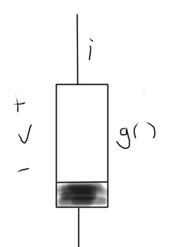
We will start off considering a non-linear resistor, designated within a circuit as sketched in fig. 2.

fig. 2. Non-linear resistor

Example: diode, with \( i = g(v) \), such as

\begin{equation}\label{eqn:multiphysicsL11:280}
i = I_0 \lr{ e^{v/{\eta V_T}} – 1 }.
\end{equation}

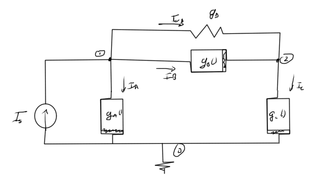
Consider the example circuit of fig. 3. KCL’s at each of the nodes are

fig. 3. Example circuit

1. \( I_A + I_B + I_D – I_s = 0 \)
2. \( – I_B + I_C – I_D = 0 \)

Introducing the consistuative equations this is

1. \( g_A(V_1) + g_B(V_1 – V_2) + g_D (V_1 – V_2) – I_s = 0 \)
2. \( – g_B(V_1 – V_2) + g_C(V_2) – g_D (V_1 – V_2) = 0 \)

In matrix form this is
\begin{equation}\label{eqn:multiphysicsL11:300}
\begin{bmatrix}
g_D & -g_D \\
-g_D & g_D
\end{bmatrix}
\begin{bmatrix}
V_1 \\
V_2
\end{bmatrix}
+
\begin{bmatrix}
g_A(V_1) &+ g_B(V_1 – V_2) & & – I_s \\
&- g_B(V_1 – V_2) & + g_C(V_2) & \\
\end{bmatrix}
=
0
.
\end{equation}

We can write the entire system as

\begin{equation}\label{eqn:multiphysicsL11:320}
\boxed{
F(\Bx) = G \Bx + F'(\Bx) = 0.
}
\end{equation}

The first term, a product of a nodal matrix \( G \) represents the linear subnetwork, and is filled with the stamps we are already familiar with.

The second term encodes the relationships of the nonlinear subnetwork. This non-linear component has been marked with a prime to distinguish it from the complete network function that includes both linear and non-linear elements.

Observe the similarity with the stamp analysis that we did previously. With \( g_A() \) connected on one end to ground we have it only once in the resulting vector, whereas the nonlinear elements connected to two non-zero nodes in the network occur once with each sign.

Stamp for nonlinear resistor

For the non-linear circuit element of fig. 4.

fig. 4. Non-linear resistor circuit element

The stamp is

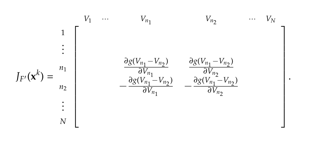
Stamp for Jacobian

\begin{equation}\label{eqn:multiphysicsL11:360}
J_F(\Bx^k) = G + J_{F’}(\Bx^k).
\end{equation}

Here the stamp for the Jacobian, an \( N \times N \) matrix, is