[Click here for a PDF of this post with nicer formatting]
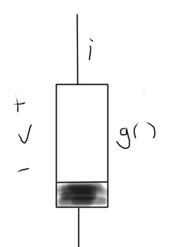
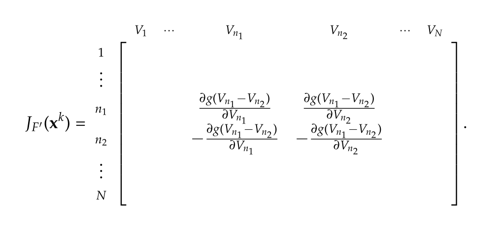
Because it was simple, a coordinate expansion of the Jacobian of the non-linear currents was good to get a feeling for the structure of the equations. However, a Jacobian of that form is impossibly slow to compute for larger \( N \). It seems plausible that eliminating the coordinate expansion, expressing both the currrent and the Jacobian directly in terms of the Harmonic Balance unknowns vector \( \BV \), would lead to a simpler set of equations that could be implemented in a computationally more effective way. To aid in this discovery, consider the simple RC load diode circuit of fig. 1. It’s not too hard to start from scratch with the time domain nodal equations for this circuit, which are
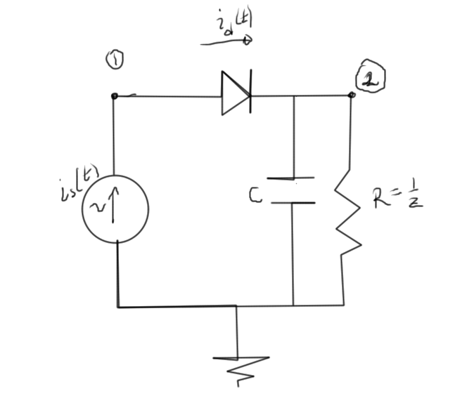
fig. 1. Simple diode and resistor circuit
- \( 0 = i_s – i_d \)
- \( Z v^{(2)} + C dv^{(2)}/dt = i_d \)
- \( i_d = I_0 \lr{ e^{(v^{(1)} – v^{(2)})/V_T} – 1} \)
To setup for matrix form, let
\begin{equation}\label{eqn:diodeRLCSample:1240}
\Bv(t) =
\begin{bmatrix}
v^{(1)}(t) \\
v^{(2)}(t) \\
\end{bmatrix}
\end{equation}
\begin{equation}\label{eqn:diodeRLCSample:1140}
\BG =
\begin{bmatrix}
0 & 0 \\
0 & Z \\
\end{bmatrix}
\end{equation}
\begin{equation}\label{eqn:diodeRLCSample:1160}
\BC =
\begin{bmatrix}
0 & 0 \\
0 & C \\
\end{bmatrix}
\end{equation}
\begin{equation}\label{eqn:diodeRLCSample:1180}
\Bd =
\begin{bmatrix}
1 \\
-1
\end{bmatrix}
\end{equation}
\begin{equation}\label{eqn:diodeRLCSample:1200}
\Bb =
\begin{bmatrix}
1 \\
0
\end{bmatrix},
\end{equation}
so that the time domain equations can be written as
\begin{equation}\label{eqn:diodeRLCSample:1220}
\BG \Bv(t)
+ \BC \Bv'(t)
=
\Bb i_s(t)
+
I_0
\Bd
\lr{
e^{ (v^{(1)}(t) – v^{(2)}(t))/V_T} – 1
}
=
\begin{bmatrix}
\Bb & -I_0 \Bd
\end{bmatrix}
\begin{bmatrix}
i_s(t) \\
1
\end{bmatrix}
+
I_0 \Bd
e^{ (v^{(1)}(t) – v^{(2)}(t))/V_T}.
\end{equation}
Harmonic Balance is essentially the assumption that the input and outputs are assumed to be a bandwidth limited periodic signal, and the non-linear components can be approximated by the same
\begin{equation}\label{eqn:diodeRLCSample:1260}
i_s(t) = \sum_{n=-N}^N I^{(s)}_n e^{ j \omega_0 n t },
\end{equation}
\begin{equation}\label{eqn:diodeRLCSample:1280}
v^{(k)}(t) =
\sum_{n=-N}^N V^{(k)}_n e^{ j \omega_0 n t },
\end{equation}
\begin{equation}\label{eqn:diodeRLCSample:1300}
\epsilon(t) =
e^{ (v^{(1)}(t) – v^{(2)}(t))/V_T}
\simeq
\sum_{n=-N}^N E_n e^{ j \omega_0 n t },
\end{equation}
The approximation in \ref{eqn:diodeRLCSample:1300} is an equality only at the Nykvist sampling times \( t_k = T k/(2 N + 1) \). The Fourier series provides a periodic extension to other times that will approximate the underlying periodic non-linear relation.
With all the time dependence locked into the exponentials, the derivatives are really easy to calculate
\begin{equation}\label{eqn:diodeRLCSample:1281}
\frac{d}{dt} v^{(k)}(t) =
\sum_{n=-N}^N j \omega_0 n V^{(k)}_n e^{ j \omega_0 n t }.
\end{equation}
Inserting all of these into \ref{eqn:diodeRLCSample:1220} gives
\begin{equation}\label{eqn:diodeRLCSample:1320}
\sum_{n=-N}^N e^{ j \omega_0 n t} \lr{ \BG + j \omega_0 n \BC }
\begin{bmatrix}
V^{(1)}_n \\
V^{(2)}_n \\
\end{bmatrix}
=
\sum_{n=-N}^N e^{ j \omega_0 n t}
\lr{
-I_0 \Bd \delta_{n 0}
+
\Bb I^{(s)}_n
+ I_0 \Bd E_n
}.
\end{equation}
The periodic assumption requires equality for each \( e^{j \omega_0 n t} \), or
\begin{equation}\label{eqn:diodeRLCSample:1340}
\lr{ \BG + j \omega_0 n \BC }
\begin{bmatrix}
V^{(1)}_n \\
V^{(2)}_n \\
\end{bmatrix}
=
-I_0 \Bd \delta_{n 0}
+
\Bb I^{(s)}_n
+ I_0 \Bd E_n.
\end{equation}
For illustration, consider the \( N = 1 \) case, where the block matrix form is
\begin{equation}\label{eqn:diodeRLCSample:1360}
\begin{bmatrix}
\BG + j \omega_0 (-1) \BC & 0 & 0 \\
0 & \BG + j \omega_0 (0) \BC & 0 \\
0 & 0 & \BG + j \omega_0 (1) \BC
\end{bmatrix}
\begin{bmatrix}
\begin{bmatrix}
V^{(1)}_{-1} \\
V^{(2)}_{-1} \\
\end{bmatrix} \\
\begin{bmatrix}
V^{(1)}_{0} \\
V^{(2)}_{0} \\
\end{bmatrix} \\
\begin{bmatrix}
V^{(1)}_{1} \\
V^{(2)}_{1} \\
\end{bmatrix}
\end{bmatrix}
=
\begin{bmatrix}
\Bb I^{(s)}_{-1} \\
\Bb I^{(s)}_{0} – I_0 \Bd \\
\Bb I^{(s)}_{1} \\
\end{bmatrix}
+
I_0
\begin{bmatrix}
\Bd E_{-1} \\
\Bd E_{0} \\
\Bd E_{1} \\
\end{bmatrix}.
\end{equation}
The structure of this equation is
\begin{equation}\label{eqn:diodeRLCSample:1380}
\BY \BV = \BI + \mathcal{I}(\BV),
\end{equation}
The non-linear current \( \mathcal{I}(\BV) \) needs to be examined further. How much of this can be precomputed, and what is the simplest way to compute the Jacobian? With
\begin{equation}\label{eqn:diodeRLCSample:1400}
\BE =
\begin{bmatrix}
E_{-1} \\
E_{0} \\
E_{1} \\
\end{bmatrix}, \qquad
\Bepsilon =
\begin{bmatrix}
\epsilon_{-1} \\
\epsilon_{0} \\
\epsilon_{1} \\
\end{bmatrix},
\end{equation}
the non-linear current is
\begin{equation}\label{eqn:diodeRLCSample:1420}
\mathcal{I} =
I_0
\begin{bmatrix}
\Bd E_{-1} \\
\Bd E_{0} \\
\Bd E_{1} \\
\end{bmatrix}
=
I_0
\begin{bmatrix}
\Bd \begin{bmatrix} 1 & 0 & 0 \end{bmatrix} \BE \\
\Bd \begin{bmatrix} 0 & 1 & 0 \end{bmatrix} \BE \\
\Bd \begin{bmatrix} 0 & 0 & 1 \end{bmatrix} \BE
\end{bmatrix}
=
I_0
\begin{bmatrix}
\Bd & 0 & 0 \\
0 & \Bd & 0 \\
0 & 0 & \Bd
\end{bmatrix}
\BF^{-1} \Bepsilon
\end{equation}
In the last step \( \BE = \BF^{-1} \Bepsilon \) has been factored out (in its inverse Fourier form). With
\begin{equation}\label{eqn:diodeRLCSample:1480}
\BD =
\begin{bmatrix}
\Bd & 0 & 0 \\
0 & \Bd & 0 \\
0 & 0 & \Bd \\
\end{bmatrix},
\end{equation}
the current is
\begin{equation}\label{eqn:diodeRLCSample:1540}
\boxed{
\mathcal{I}(\BV) =
I_0 \BD \BF^{-1} \Bepsilon(\BV).
}
\end{equation}
The next step is finding an appropriate form for \( \Bepsilon \)
\begin{equation}\label{eqn:diodeRLCSample:1440}
\begin{aligned}
\Bepsilon &=
\begin{bmatrix}
\epsilon(t_{-1}) \\
\epsilon(t_{0}) \\
\epsilon(t_{1}) \\
\end{bmatrix} \\
&=
\begin{bmatrix}
\exp\lr{ \lr{ v^{(1)}_{-1} – v^{(2)}_{-1} }/V_T } \\
\exp\lr{ \lr{ v^{(1)}_{0} – v^{(2)}_{0} }/V_T } \\
\exp\lr{ \lr{ v^{(1)}_{1} – v^{(2)}_{1} }/V_T }
\end{bmatrix} \\
&=
\begin{bmatrix}
\exp\lr{
\begin{bmatrix}
1 & 0 & 0
\end{bmatrix}
\lr{ \Bv^{(1)} – \Bv^{(2)} }/V_T } \\
\exp\lr{
\begin{bmatrix}
0 & 1 & 0
\end{bmatrix}
\lr{ \Bv^{(1)} – \Bv^{(2)} }/V_T } \\
\exp\lr{
\begin{bmatrix}
0 & 0 & 1
\end{bmatrix}
\lr{ \Bv^{(1)} – \Bv^{(2)} }/V_T } \\
\end{bmatrix} \\
&=
\begin{bmatrix}
\exp\lr{
\begin{bmatrix}
1 & 0 & 0
\end{bmatrix}
\BF
\lr{ \BV^{(1)} – \BV^{(2)} }/V_T } \\
\exp\lr{
\begin{bmatrix}
0 & 1 & 0
\end{bmatrix}
\BF
\lr{ \BV^{(1)} – \BV^{(2)} }/V_T } \\
\exp\lr{
\begin{bmatrix}
0 & 0 & 1
\end{bmatrix}
\BF
\lr{ \BV^{(1)} – \BV^{(2)} }/V_T } \\
\end{bmatrix}.
\end{aligned}
\end{equation}
It would be nice to have the difference of frequency domain vectors expressed in terms of \( \BV \), which can be done with a bit of rearrangement
\begin{equation}\label{eqn:diodeRLCSample:1460}
\begin{aligned}
\BV^{(1)} – \BV^{(2)}
&=
\begin{bmatrix}
V^{(1)}_{-1} – V^{(2)}_{-1} \\
V^{(1)}_{0} – V^{(2)}_{0} \\
V^{(1)}_{1} – V^{(2)}_{1} \\
\end{bmatrix} \\
&=
\begin{bmatrix}
1 & -1 & 0 & 0 & 0 & 0 \\
0 & 0 & 1 & -1 & 0 & 0 \\
0 & 0 & 0 & 0 & 1 & -1 \\
\end{bmatrix}
\begin{bmatrix}
V_{-1}^{(1)} \\
V_{-1}^{(2)} \\
V_{0}^{(1)} \\
V_{0}^{(2)} \\
V_{1}^{(1)} \\
V_{1}^{(2)} \\
\end{bmatrix} \\
&=
\begin{bmatrix}
\Bd^\T & 0 & 0 \\
0 & \Bd^\T & 0 \\
0 & 0 & \Bd^\T \\
\end{bmatrix}
\BV \\
&= \BD^\T \BV,
\end{aligned}
\end{equation}
\begin{equation}\label{eqn:diodeRLCSample:1520}
\BH
=
\BF \BD^\T /V_T
=
\begin{bmatrix}
\Bh_1^\T \\
\Bh_2^\T \\
\Bh_3^\T
\end{bmatrix},
\end{equation}
which allows the non-linear current to can now be completely expressed in terms of \( \BV \).
\begin{equation}\label{eqn:diodeRLCSample:1560}
\boxed{
\Bepsilon(\BV)
=
\begin{bmatrix}
e^{\Bh_1^\T \BV} \\
e^{\Bh_2^\T \BV} \\
e^{\Bh_3^\T \BV} \\
\end{bmatrix}.
}
\end{equation}
Jacobian
With a compact matrix representation of the non-linear current, attention can now be turned to the Jacobian of the non-linear current. Let \( \BA = I_0 \BD \BF^{-1} = [ a_{ij} ]_{ij} \), the current (with summation implied) is
\begin{equation}\label{eqn:diodeRLCSample:1580}
\mathcal{I} =
\begin{bmatrix}
a_{ik} \epsilon_k,
\end{bmatrix}
\end{equation}
with coordinates
\begin{equation}\label{eqn:diodeRLCSample:1600}
\mathcal{I}_i = a_{ik} \epsilon_k = a_{ik} \exp\lr{ \Bh_k^\T \BV }.
\end{equation}
so the Jacobian components are
\begin{equation}\label{eqn:diodeRLCSample:1620}
[\BJ^{\mathcal{I}}]_{ij}
=
a_{ik} \epsilon_k = a_{ik}
\PD{V_j}{}
\exp\lr{ \Bh_k^\T \BV }
=
a_{ik}
h_{kj}
\exp\lr{ \Bh_k^\T \BV }.
\end{equation}
Factoring out \( \BU = [h_{ij} \exp\lr{ \Bh_i^\T \BV }]_{ij} \),
\begin{equation}\label{eqn:diodeRLCSample:1640}
\BJ^{\mathcal{I}}
= \BA \BU
=
\BA
\begin{bmatrix}
\begin{bmatrix} h_{11} & h_{12} & \cdots h_{1, R(2 N + 1)}\end{bmatrix} \exp\lr{ \Bh_1^\T \BV } \\
\begin{bmatrix} h_{21} & h_{22} & \cdots h_{2, R(2 N + 1)}\end{bmatrix} \exp\lr{ \Bh_2^\T \BV } \\
\begin{bmatrix} h_{31} & h_{32} & \cdots h_{3, R(2 N + 1)}\end{bmatrix} \exp\lr{ \Bh_3^\T \BV } \\
\end{bmatrix}
=
\BA
\begin{bmatrix}
\Bh_1^\T \exp\lr{ \Bh_1^\T \BV } \\
\Bh_2^\T \exp\lr{ \Bh_2^\T \BV } \\
\Bh_3^\T \exp\lr{ \Bh_3^\T \BV } \\
\end{bmatrix}.
\end{equation}
A quick sanity check of dimensions seems worthwhile, and shows that all is well
- \( \BA \) : \( R(2 N + 1) \times 2 N + 1 \)
- \( \BU \) : \( 2 N + 1 \times R(2 N + 1) \)
- \( \BJ^{\mathcal{I}} \) : \( R(2 N + 1) \times R(2 N + 1) \)
The Jacobian of the non-linear current is now completely determined
\begin{equation}\label{eqn:diodeRLCSample:1660}
\boxed{
\BJ^{\mathcal{I}}( \BV ) =
I_0 \BD \BF^{-1}
\begin{bmatrix}
\Bh_1^\T \exp\lr{ \Bh_1^\T \BV } \\
\Bh_2^\T \exp\lr{ \Bh_2^\T \BV } \\
\Bh_3^\T \exp\lr{ \Bh_3^\T \BV } \\
\end{bmatrix}.
}
\end{equation}
Newton’s method solution
All the pieces required for a Newton’s method solution are now in place. The goal is to find a value of \( \BV \) that provides the zero
\begin{equation}\label{eqn:diodeRLCSample:1680}
f(\BV) = \BY \BV – \BI – \mathcal{I}(\BV).
\end{equation}
Expansion to first order around an initial guess \( \BV^0 \), gives
\begin{equation}\label{eqn:diodeRLCSample:1700}
f( \BV^0 + \Delta \BV ) = f(\BV^0) + \BJ(\BV^0) \Delta \BV \approx 0,
\end{equation}
where the full Jacobian of \( f(\BV) \) is
\begin{equation}\label{eqn:diodeRLCSample:1720}
\BJ(\BV) = \BY – \BJ^{\mathcal{I}}(\BV).
\end{equation}
The Newton’s method refinement of the initial guess follows by inversion
\begin{equation}\label{eqn:diodeRLCSample:1740}
\Delta \BV = -\lr{ \BY – \BJ^{\mathcal{I}}(\BV^0) }^{-1} f(\BV^0).
\end{equation}