[Click here for a PDF of this post with nicer formatting]
Disclaimer
Peeter’s lecture notes from class. These may be incoherent and rough.
These are notes for the UofT course PHY1520, Graduate Quantum Mechanics, taught by Prof. Paramekanti, covering [1] chap. 3 content.
Review: Angular momentum
Given eigenket \( \ket{a, b} \), where
\begin{equation}\label{eqn:qmLecture14:20}
\begin{aligned}
\hat{\BL}^2 \ket{a, b} &= \Hbar^2 a \ket{a,b} \\
\hat{L}_z \ket{a, b} &= \Hbar b \ket{a,b}
\end{aligned}
\end{equation}
We were looking for
\begin{equation}\label{eqn:qmLecture14:40}
\hat{L}_{x,y} \ket{a,b} = \sum_{b’} \mathcal{A}^{x,y}_{a; b, b’} \ket{a,b’},
\end{equation}
by applying
\begin{equation}\label{eqn:qmLecture14:60}
\hat{L}_{\pm} = \hat{L}_x \pm i \hat{L}_y.
\end{equation}
We found
\begin{equation}\label{eqn:qmLecture14:80}
\hat{L}_{\pm} \propto \ket{a, b \pm 1}.
\end{equation}
Let
\begin{equation}\label{eqn:qmLecture14:100}
\ket{\phi_\pm} = \hat{L}_{\pm} \ket{a, b}.
\end{equation}
We want
\begin{equation}\label{eqn:qmLecture14:120}
\braket{\phi_\pm}{\phi_\pm} \ge 0,
\end{equation}
or
\begin{equation}\label{eqn:qmLecture14:140}
\begin{aligned}
\bra{a,b} \hat{L}_{+} \hat{L}_{-} \ket{a, b} &\ge 0 \\
\bra{a,b} \hat{L}_{-} \hat{L}_{+} \ket{a, b} &\ge 0
\end{aligned}
\end{equation}
We found
\begin{equation}\label{eqn:qmLecture14:160}
\begin{aligned}
\hat{L}_{+} \hat{L}_{-} =
\lr{ \hat{L}_x + i \hat{L}_y } \lr{ \hat{L}_x – i \hat{L}_y }
&= \lr{ \hat{\BL}^2 – \hat{L}_z^2 } -i \antisymmetric{\hat{L}_x}{\hat{L}_y} \\
&= \lr{ \hat{\BL}^2 – \hat{L}_z^2 } -i \lr{ i \Hbar \hat{L}_z } \\
&= \lr{ \hat{\BL}^2 – \hat{L}_z^2 } + \Hbar \hat{L}_z,
\end{aligned}
\end{equation}
so
\begin{equation}\label{eqn:qmLecture14:180}
\bra{a,b} \hat{L}_{+} \hat{L}_{-} \ket{a, b}
=
\expectation{ \hat{\BL}^2 – \hat{L}_z^2 + \Hbar \hat{L}_z }.
\end{equation}
Similarly
\begin{equation}\label{eqn:qmLecture14:200}
\bra{a,b} \hat{L}_{-} \hat{L}_{+} \ket{a, b}
=
\expectation{ \hat{\BL}^2 – \hat{L}_z^2 – \Hbar \hat{L}_z }.
\end{equation}
Constraints
\begin{equation}\label{eqn:qmLecture14:220}
\begin{aligned}
a – b^2 + b &\ge 0 \\
a – b^2 – b &\ge 0
\end{aligned}
\end{equation}
If these are satisfied at the equality extreme we have
\begin{equation}\label{eqn:qmLecture14:240}
\begin{aligned}
b_{\textrm{max}} \lr{ b_{\textrm{max}} + 1 } &= a \\
b_{\textrm{min}} \lr{ b_{\textrm{min}} – 1 } &= a.
\end{aligned}
\end{equation}
Rearranging this to solve, we can rewrite the equality as
\begin{equation}\label{eqn:qmLecture14:680}
\lr{ b_{\textrm{max}} + \inv{2} }^2 – \inv{4} = \lr{ b_{\textrm{min}} – \inv{2} }^2 – \inv{4},
\end{equation}
which has solutions at
\begin{equation}\label{eqn:qmLecture14:700}
b_{\textrm{max}} + \inv{2} = \pm \lr{ b_{\textrm{min}} – \inv{2} }.
\end{equation}
One of the solutions is
\begin{equation}\label{eqn:qmLecture14:260}
-b_{\textrm{min}} = b_{\textrm{max}}.
\end{equation}
The other solution is \( b_{\textrm{max}} = b_{\textrm{min}} – 1 \), which we discard.
The final constraint is therefore
\begin{equation}\label{eqn:qmLecture14:280}
\boxed{
– b_{\textrm{max}} \le b \le b_{\textrm{max}},
}
\end{equation}
and
\begin{equation}\label{eqn:qmLecture14:320}
\begin{aligned}
\hat{L}_{+} \ket{a, b_{\textrm{max}}} &= 0 \\
\hat{L}_{-} \ket{a, b_{\textrm{min}}} &= 0
\end{aligned}
\end{equation}
If we had the sequence, which must terminate at \( b_{\textrm{min}} \) or else it will go on forever
\begin{equation}\label{eqn:qmLecture14:340}
\ket{a, b_{\textrm{max}}}
\overset{\hat{L}_{-}}{\rightarrow}
\ket{a, b_{\textrm{max}} – 1}
\overset{\hat{L}_{-}}{\rightarrow}
\ket{a, b_{\textrm{max}} – 2}
\cdots
\overset{\hat{L}_{-}}{\rightarrow}
\ket{a, b_{\textrm{min}}},
\end{equation}
then we know that \( b_{\textrm{max}} – b_{\textrm{min}} \in \mathbb{Z} \), or
\begin{equation}\label{eqn:qmLecture14:360}
b_{\textrm{max}} – n = b_{\textrm{min}} = -b_{\textrm{max}}
\end{equation}
or
\begin{equation}\label{eqn:qmLecture14:380}
b_{\textrm{max}} = \frac{n}{2},
\end{equation}
this is either an integer or a \( 1/2 \) odd integer, depending on whether \( n \) is even or odd. These are called “orbital” or “spin” respectively.
The convention is to write
\begin{equation}\label{eqn:qmLecture14:400}
\begin{aligned}
b_{\textrm{max}} &= j \\
a &= j(j + 1).
\end{aligned}
\end{equation}
so for \( m \in -j, -j + 1, \cdots, +j \)
\begin{equation}\label{eqn:qmLecture14:420}
\boxed{
\begin{aligned}
\hat{\BL}^2 \ket{j, m} &= \Hbar^2 j (j + 1) \ket{j, m} \\
L_z \ket{j, m} &= \Hbar m \ket{j, m}.
\end{aligned}
}
\end{equation}
Schwinger’s Harmonic oscillator representation of angular momentum operators.
In [2] a powerful method for describing angular momentum with harmonic oscillators was introduced, which will be outlined here. The question is whether we can construct a set of harmonic oscillators that allows a mapping from
\begin{equation}\label{eqn:qmLecture14:460}
\hat{L}_{+} \leftrightarrow a^{+}?
\end{equation}
Picture two harmonic oscillators, one with states counted from one zero towards \( \infty \) and another with states counted from a different zero towards \( -\infty \), as pictured in fig. 1.
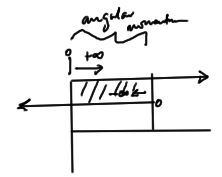
fig. 1. Overlapping SHO domains
Is it possible that such an overlapping set of harmonic oscillators can provide the properties of the angular momentum operators? Let’s relabel the counting so that we have two sets of positive counted SHO systems, each counted in a positive direction as sketched in fig. 2.
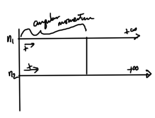
fig. 2. Relabeling the counting for overlapping SHO systems
It turns out that given a constraint there the number of ways to distribute particles between a pair of SHO systems, the process that can be viewed as reproducing the angular momentum action is a transfer of particles from one harmonic oscillator to the other. For \( \hat{L}_z = +j \)
\begin{equation}\label{eqn:qmLecture14:480}
\begin{aligned}
n_1 &= n_{\textrm{max}} \\
n_2 &= 0,
\end{aligned}
\end{equation}
and for \( \hat{L}_z = -j \)
\begin{equation}\label{eqn:qmLecture14:500}
\begin{aligned}
n_1 &= 0 \\
n_2 &= n_{\textrm{max}}.
\end{aligned}
\end{equation}
We can make the identifications
\begin{equation}\label{eqn:qmLecture14:520}
\hat{L}_z = \lr{ n_1 – n_2 } \frac{\Hbar}{2},
\end{equation}
and
\begin{equation}\label{eqn:qmLecture14:540}
j = \inv{2} n_{\textrm{max}},
\end{equation}
or
\begin{equation}\label{eqn:qmLecture14:560}
n_1 + n_2 = \text{fixed} = n_{\textrm{max}}
\end{equation}
Changes that keep \( n_1 + n_2 \) fixed are those that change \( n_1 \), \( n_2 \) by \( +1 \) or \( -1 \) respectively, as sketched in fig. 3.
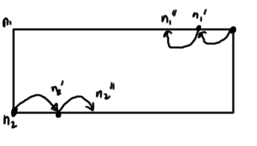
fig. 3. Number conservation constraint.
Can we make an identification that takes
\begin{equation}\label{eqn:qmLecture14:580}
\ket{n_1, n_2} \overset{\hat{L}_{-}}{\rightarrow} \ket{n_1 – 1, n_2 + 1}?
\end{equation}
What operator in the SHO problem has this effect? Let’s try
\boxedEquation{eqn:qmLecture14:620}{
\begin{aligned}
\hat{L}_{-} &= \Hbar a_2^\dagger a_1 \\
\hat{L}_{+} &= \Hbar a_1^\dagger a_2 \\
\hat{L}_z &= \frac{\Hbar}{2} \lr{ n_1 – n_2 }
\end{aligned}
}
Is this correct? Do we need to make any scalar adjustments? We want
\begin{equation}\label{eqn:qmLecture14:640}
\antisymmetric{\hat{L}_z}{\hat{L}_{\pm}} = \pm \Hbar \hat{L}_{\pm}.
\end{equation}
First check this with the \( \hat{L}_{+} \) commutator
\begin{equation}\label{eqn:qmLecture14:660}
\begin{aligned}
\antisymmetric{\hat{L}_z}{\hat{L}_{+}}
&=
\inv{2} \Hbar^2 \antisymmetric{ n_1 – n_2}{a_1^\dagger a_2 } \\
&=
\inv{2} \Hbar^2 \antisymmetric{ a_1^\dagger a_1 – a_2^\dagger a_2 }{a_1^\dagger a_2 } \\
&=
\inv{2} \Hbar^2
\lr{
\antisymmetric{ a_1^\dagger a_1 }{a_1^\dagger a_2 }
-\antisymmetric{ a_2^\dagger a_2 }{a_1^\dagger a_2 }
} \\
&=
\inv{2} \Hbar^2
\lr{
a_2 \antisymmetric{ a_1^\dagger a_1 }{a_1^\dagger }
-a_1^\dagger \antisymmetric{ a_2^\dagger a_2 }{a_2 }
}.
\end{aligned}
\end{equation}
But
\begin{equation}\label{eqn:qmLecture14:720}
\begin{aligned}
\antisymmetric{ a^\dagger a }{a^\dagger }
&=
a^\dagger a
a^\dagger
–
a^\dagger
a^\dagger a \\
&=
a^\dagger \lr{ 1 +
a^\dagger a}
–
a^\dagger
a^\dagger a \\
&=
a^\dagger,
\end{aligned}
\end{equation}
and
\begin{equation}\label{eqn:qmLecture14:740}
\begin{aligned}
\antisymmetric{ a^\dagger a }{a}
&=
a^\dagger a a
-a a^\dagger a \\
&=
a^\dagger a a
-\lr{ 1 + a^\dagger a } a \\
&=
-a,
\end{aligned}
\end{equation}
so
\begin{equation}\label{eqn:qmLecture14:760}
\antisymmetric{\hat{L}_z}{\hat{L}_{+}} = \Hbar^2 a_2 a_1^\dagger = \Hbar \hat{L}_{+},
\end{equation}
as desired. Similarly
\begin{equation}\label{eqn:qmLecture14:780}
\begin{aligned}
\antisymmetric{\hat{L}_z}{\hat{L}_{-}}
&=
\inv{2} \Hbar^2 \antisymmetric{ n_1 – n_2}{a_2^\dagger a_1 } \\
&=
\inv{2} \Hbar^2 \antisymmetric{ a_1^\dagger a_1 – a_2^\dagger a_2 }{a_2^\dagger a_1 } \\
&=
\inv{2} \Hbar^2 \lr{
a_2^\dagger \antisymmetric{ a_1^\dagger a_1 }{a_1 }
– a_1 \antisymmetric{ a_2^\dagger a_2 }{a_2^\dagger }
} \\
&=
\inv{2} \Hbar^2 \lr{
a_2^\dagger (-a_1)
– a_1 a_2^\dagger
} \\
&=
– \Hbar^2 a_2^\dagger a_1 \\
&=
– \Hbar \hat{L}_{-}.
\end{aligned}
\end{equation}
With
\begin{equation}\label{eqn:qmLecture14:800}
\begin{aligned}
j &= \frac{n_1 + n_2}{2} \\
m &= \frac{n_1 – n_2}{2} \\
\end{aligned}
\end{equation}
We can make the identification
\begin{equation}\label{eqn:qmLecture14:820}
\ket{n_1, n_2} = \ket{ j+ m , j – m}.
\end{equation}
Another way
With
\begin{equation}\label{eqn:qmLecture14:840}
\hat{L}_{+} \ket{j, m} = d_{j,m}^{+} \ket{j, m+1}
\end{equation}
or
\begin{equation}\label{eqn:qmLecture14:860}
\Hbar a_1^\dagger a_2 \ket{j + m, j-m} = d_{j,m}^{+} \ket{ j + m + 1, j- m-1},
\end{equation}
we can seek this factor \( d_{j,m}^{+} \) by operating with \( \hat{L}_{+} \)
\begin{equation}\label{eqn:qmLecture14:880}
\begin{aligned}
\hat{L}_{+} \ket{j, m}
&=
\Hbar a_1^\dagger a_2 \ket{n_1, n_2} \\
&=
\Hbar a_1^\dagger a_2 \ket{j+m,j-m} \\
&=
\Hbar \sqrt{ n + 1 } \sqrt{n_2} \ket{j+m +1,j-m-1} \\
&=
\Hbar \sqrt{ \lr{ j+ m + 1}\lr{ j – m } } \ket{j+m +1,j-m-1}
\end{aligned}
\end{equation}
That gives
\begin{equation}\label{eqn:qmLecture14:900}
\begin{aligned}
d_{j,m}^{+} &= \Hbar \sqrt{\lr{ j – m } \lr{ j+ m + 1} } \\
d_{j,m}^{-} &= \Hbar \sqrt{\lr{ j + m } \lr{ j- m + 1} }.
\end{aligned}
\end{equation}
This equivalence can be used to model spin interaction in crystals as harmonic oscillators. This equivalence of lattice vibrations and spin oscillations is called “spin waves”.
References
[1] Jun John Sakurai and Jim J Napolitano. Modern quantum mechanics. Pearson Higher Ed, 2014.
[2] J Schwinger. Quantum theory of angular momentum. biedenharn l., van dam h., editors, 1955. URL http://www.ifi.unicamp.br/ cabrera/teaching/paper_schwinger.pdf.