[Click here for a PDF of this post with nicer formatting]
Here’s a simple problem, a lot like the problem set 6 variational calculation.
Q: [1] 5.21
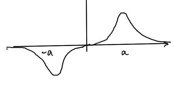
Estimate the lowest eigenvalue \( \lambda \) of the differential equation
\begin{equation}\label{eqn:absolutePotentialVariation:20}
\frac{d^2}{dx^2}\psi + \lr{ \lambda – \Abs{x} } \psi = 0.
\end{equation}
Using \( \alpha \) variation with the trial function
\begin{equation}\label{eqn:absolutePotentialVariation:40}
\psi =
\left\{
\begin{array}{l l}
c(\alpha – \Abs{x}) & \quad \mbox{\(\Abs{x} < \alpha \) } \\
0 & \quad \mbox{\(\Abs{x} > \alpha \) }
\end{array}
\right.
\end{equation}
A:
First rewrite the differential equation in a Hamiltonian like fashion
\begin{equation}\label{eqn:absolutePotentialVariation:60}
H \psi = -\frac{d^2}{dx^2}\psi + \Abs{x} \psi = \lambda \psi.
\end{equation}
We need the derivatives of the trial distribution. The first derivative is
\begin{equation}\label{eqn:absolutePotentialVariation:80}
\begin{aligned}
\frac{d}{dx} \psi
&=
-c \frac{d}{dx} \Abs{x} \\
&=
-c \frac{d}{dx} \lr{ x \theta(x) – x \theta(-x) } \\
&=
-c \lr{
\theta(x) – \theta(-x)
+
x \delta(x) + x \delta(-x)
} \\
&=
-c \lr{
\theta(x) – \theta(-x)
+
2 x \delta(x)
}.
\end{aligned}
\end{equation}
The second derivative is
\begin{equation}\label{eqn:absolutePotentialVariation:100}
\begin{aligned}
\frac{d^2}{dx^2} \psi
&=
-c \frac{d}{dx} \lr{
\theta(x) – \theta(-x)
+
2 x \delta(x)
} \\
&=
-c \lr{
\delta(x) + \delta(-x)
+
2 \delta(x)
+
2 x \delta'(x)
} \\
&=
-c \lr{
4 \delta(x)
+
2 x \frac{-\delta(x) }{x}
} \\
&=
-2 c \delta(x).
\end{aligned}
\end{equation}
This gives
\begin{equation}\label{eqn:absolutePotentialVariation:120}
H \psi = -2 c \delta(x) + \Abs{x} c \lr{ \alpha – \Abs{x} }.
\end{equation}
We are now set to compute some of the inner products. The normalization is the simplest
\begin{equation}\label{eqn:absolutePotentialVariation:140}
\begin{aligned}
\braket{\psi}{\psi}
&= c^2 \int_{-\alpha}^\alpha ( \alpha – \Abs{x} )^2 dx \\
&= 2 c^2 \int_{0}^\alpha ( x – \alpha )^2 dx \\
&= 2 c^2 \int_{-\alpha}^0 u^2 du \\
&= 2 c^2 \lr{ -\frac{(-\alpha)^3}{3} } \\
&= \frac{2}{3} c^2 \alpha^3.
\end{aligned}
\end{equation}
For the energy
\begin{equation}\label{eqn:absolutePotentialVariation:160}
\begin{aligned}
\braket{\psi}{H \psi}
&=
c^2 \int dx \lr{ \alpha – \Abs{x} } \lr{ -2 \delta(x) + \Abs{x} \lr{ \alpha – \Abs{x} } } \\
&=
c^2 \lr{ – 2 \alpha + \int_{-\alpha}^\alpha dx \lr{ \alpha – \Abs{x} }^2 \Abs{x} } \\
&=
c^2 \lr{ – 2 \alpha + 2 \int_{-\alpha}^0 du u^2 \lr{ u + \alpha } } \\
&=
c^2 \lr{ – 2 \alpha + 2 \evalrange{\lr{ \frac{u^4}{4} + \alpha \frac{u^3}{3} }}{-\alpha}{0} } \\
&=
c^2 \lr{ – 2 \alpha – 2 \lr{ \frac{\alpha^4}{4} – \frac{\alpha^4}{3} } } \\
&=
c^2 \lr{ – 2 \alpha + \inv{6} \alpha^4 }.
\end{aligned}
\end{equation}
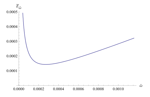
The energy estimate is
\begin{equation}\label{eqn:absolutePotentialVariation:180}
\begin{aligned}
\overline{{E}}
&=
\frac{\braket{\psi}{H \psi}}{\braket{\psi}{\psi}} \\
&=
\frac{ – 2 \alpha + \inv{6} \alpha^4 }{ \frac{2}{3} \alpha^3} \\
&=
– \frac{3}{\alpha^2} + \inv{4} \alpha.
\end{aligned}
\end{equation}
This has its minimum at
\begin{equation}\label{eqn:absolutePotentialVariation:200}
0 = -\frac{6}{\alpha^3} + \inv{4},
\end{equation}
or
\begin{equation}\label{eqn:absolutePotentialVariation:220}
\alpha = 2 \times 3^{1/3}.
\end{equation}
Back subst into the energy gives
\begin{equation}\label{eqn:absolutePotentialVariation:240}
\begin{aligned}
\overline{{E}}
&=
– \frac{3}{4 \times 3^{2/3}} + \inv{2} 3^{1/3} \\
&= \frac{3^{4/3}}{4} \\
&\approx 1.08.
\end{aligned}
\end{equation}
The problem says the exact answer is 1.019, so the variation gets within 6 %.
References
[1] Jun John Sakurai and Jim J Napolitano. Modern quantum mechanics. Pearson Higher Ed, 2014.
![fig. 2. Infinite potential [0,L] box.](https://peeterjoot.com/wp-content/uploads/2015/11/lecture18Fig2.png)
![fig. 3. Infinite potential [-L/2,L/2] box.](https://peeterjoot.com/wp-content/uploads/2015/11/lecture18Fig3.png)