Day: October 13, 2016

Vector Area

October 13, 2016 math and physics play , , , ,

[Click here for a PDF of this post with nicer formatting]

One of the results of this problem is required for a later one on magnetic moments that I’d like to do.

Question: Vector Area. ([1] pr. 1.61)

The integral

\begin{equation}\label{eqn:vectorAreaGriffiths:20}
\Ba = \int_S d\Ba,
\end{equation}

is sometimes called the vector area of the surface \( S \).

(a)

Find the vector area of a hemispherical bowl of radius \( R \).

(b)

Show that \( \Ba = 0 \) for any closed surface.

(c)

Show that \( \Ba \) is the same for all surfaces sharing the same boundary.

(d)

Show that
\begin{equation}\label{eqn:vectorAreaGriffiths:40}
\Ba = \inv{2} \oint \Br \cross d\Bl,
\end{equation}

where the integral is around the boundary line.

(e)

Show that
\begin{equation}\label{eqn:vectorAreaGriffiths:60}
\oint \lr{ \Bc \cdot \Br } d\Bl = \Ba \cross \Bc.
\end{equation}

Answer

(a)

\begin{equation}\label{eqn:vectorAreaGriffiths:80}
\begin{aligned}
\Ba
&=
\int_{0}^{\pi/2} R^2 \sin\theta d\theta \int_0^{2\pi} d\phi
\lr{ \sin\theta \cos\phi, \sin\theta \sin\phi, \cos\theta } \\
&=
R^2 \int_{0}^{\pi/2} d\theta \int_0^{2\pi} d\phi
\lr{ \sin^2\theta \cos\phi, \sin^2\theta \sin\phi, \sin\theta\cos\theta } \\
&=
2 \pi R^2 \int_{0}^{\pi/2} d\theta \Be_3
\sin\theta\cos\theta \\
&=
\pi R^2
\Be_3
\int_{0}^{\pi/2} d\theta
\sin(2 \theta) \\
&=
\pi R^2
\Be_3
\evalrange{\lr{\frac{-\cos(2 \theta)}{2}}}{0}{\pi/2} \\
&=
\pi R^2
\Be_3
\lr{ 1 – (-1) }/2 \\
&=
\pi R^2
\Be_3.
\end{aligned}
\end{equation}

(b)

As hinted in the original problem description, this follows from

\begin{equation}\label{eqn:vectorAreaGriffiths:100}
\int dV \spacegrad T = \oint T d\Ba,
\end{equation}

simply by setting \( T = 1 \).

(c)

Suppose that two surfaces sharing a boundary are parameterized by vectors \( \Bx(u, v), \Bx(a,b) \) respectively. The area integral with the first parameterization is

\begin{equation}\label{eqn:vectorAreaGriffiths:120}
\begin{aligned}
\Ba
&= \int \PD{u}{\Bx} \cross \PD{v}{\Bx} du dv \\
&= \epsilon_{ijk} \Be_i \int \PD{u}{x_j} \PD{v}{x_k} du dv \\
&=
\epsilon_{ijk} \Be_i \int
\lr{
\PD{a}{x_j}
\PD{u}{a}
+
\PD{b}{x_j}
\PD{u}{b}
}
\lr{
\PD{a}{x_k}
\PD{v}{a}
+
\PD{b}{x_k}
\PD{v}{b}
}
du dv \\
&=
\epsilon_{ijk} \Be_i \int
du dv
\lr{
\PD{a}{x_j}
\PD{u}{a}
\PD{a}{x_k}
\PD{v}{a}
+
\PD{b}{x_j}
\PD{u}{b}
\PD{b}{x_k}
\PD{v}{b}
+
\PD{b}{x_j}
\PD{u}{b}
\PD{a}{x_k}
\PD{v}{a}
+
\PD{a}{x_j}
\PD{u}{a}
\PD{b}{x_k}
\PD{v}{b}
} \\
&=
\epsilon_{ijk} \Be_i \int
du dv
\lr{
\PD{a}{x_j}
\PD{a}{x_k}
\PD{u}{a}
\PD{v}{a}
+
\PD{b}{x_j}
\PD{b}{x_k}
\PD{u}{b}
\PD{v}{b}
}
+
\epsilon_{ijk} \Be_i \int
du dv
\lr{
\PD{b}{x_j}
\PD{a}{x_k}
\PD{u}{b}
\PD{v}{a}

\PD{a}{x_k}
\PD{b}{x_j}
\PD{u}{a}
\PD{v}{b}
}.
\end{aligned}
\end{equation}

In the last step a \( j,k \) index swap was performed for the last term of the second integral. The first integral is zero, since the integrand is symmetric in \( j,k \). This leaves
\begin{equation}\label{eqn:vectorAreaGriffiths:140}
\begin{aligned}
\Ba
&=
\epsilon_{ijk} \Be_i \int
du dv
\lr{
\PD{b}{x_j}
\PD{a}{x_k}
\PD{u}{b}
\PD{v}{a}

\PD{a}{x_k}
\PD{b}{x_j}
\PD{u}{a}
\PD{v}{b}
} \\
&=
\epsilon_{ijk} \Be_i \int
\PD{b}{x_j}
\PD{a}{x_k}
\lr{
\PD{u}{b}
\PD{v}{a}

\PD{u}{a}
\PD{v}{b}
}
du dv \\
&=
\epsilon_{ijk} \Be_i \int
\PD{b}{x_j}
\PD{a}{x_k}
\frac{\partial(b,a)}{\partial(u,v)} du dv \\
&=
-\int
\PD{b}{\Bx} \cross \PD{a}{\Bx} da db \\
&=
\int
\PD{a}{\Bx} \cross \PD{b}{\Bx} da db.
\end{aligned}
\end{equation}

However, this is the area integral with the second parameterization, proving that the area-integral for any given boundary is independant of the surface.

(d)

Having proven that the area-integral for a given boundary is independent of the surface that it is evaluated on, the result follows by illustration as hinted in the full problem description. Draw a “cone”, tracing a vector \( \Bx’ \) from the origin to the position line element, and divide that cone up into infinitesimal slices as sketched in fig. 1.

conevectorareafig1

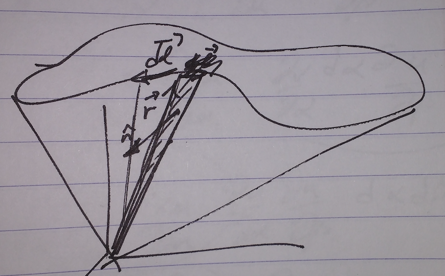
Fig 1. Cone subtended by loop

The area of each of these triangular slices is

\begin{equation}\label{eqn:vectorAreaGriffiths:160}
\inv{2} \Bx’ \cross d\Bl’.
\end{equation}

Summing those triangles proves the result.

(e)

As hinted in the problem, this follows from

\begin{equation}\label{eqn:vectorAreaGriffiths:180}
\int \spacegrad T \cross d\Ba = -\oint T d\Bl.
\end{equation}

Set \( T = \Bc \cdot \Br \), for which

\begin{equation}\label{eqn:vectorAreaGriffiths:240}
\begin{aligned}
\spacegrad T
&= \Be_k \partial_k c_m x_m \\
&= \Be_k c_m \delta_{km} \\
&= \Be_k c_k \\
&= \Bc,
\end{aligned}
\end{equation}

so
\begin{equation}\label{eqn:vectorAreaGriffiths:200}
\begin{aligned}
(\spacegrad T) \cross d\Ba
&=
\int \Bc \cross d\Ba \\
&=
\Bc \cross \int d\Ba \\
&=
\Bc \cross \Ba.
\end{aligned}
\end{equation}

so
\begin{equation}\label{eqn:vectorAreaGriffiths:220}
\Bc \cross \Ba = -\oint (\Bc \cdot \Br) d\Bl,
\end{equation}

or
\begin{equation}\label{eqn:vectorAreaGriffiths:260}
\oint (\Bc \cdot \Br) d\Bl
=
\Ba \cross \Bc.
\end{equation}

References

[1] David Jeffrey Griffiths and Reed College. Introduction to electrodynamics. Prentice hall Upper Saddle River, NJ, 3rd edition, 1999.

Magnetic moment for a localized magnetostatic current

October 13, 2016 math and physics play , , , , , , , , ,

[Click here for a PDF of this post with nicer formatting]

Motivation.

I was once again reading my Jackson [2]. This time I found that his presentation of magnetic moment didn’t really make sense to me. Here’s my own pass through it, filling in a number of details. As I did last time, I’ll also translate into SI units as I go.

Vector potential.

The Biot-Savart expression for the magnetic field can be factored into a curl expression using the usual tricks

\begin{equation}\label{eqn:magneticMomentJackson:20}
\begin{aligned}
\BB
&= \frac{\mu_0}{4\pi} \int \frac{\BJ(\Bx’) \cross (\Bx – \Bx’)}{\Abs{\Bx – \Bx’}^3} d^3 x’ \\
&= -\frac{\mu_0}{4\pi} \int \BJ(\Bx’) \cross \spacegrad \inv{\Abs{\Bx – \Bx’}} d^3 x’ \\
&= \frac{\mu_0}{4\pi} \spacegrad \cross \int \frac{\BJ(\Bx’)}{\Abs{\Bx – \Bx’}} d^3 x’,
\end{aligned}
\end{equation}

so the vector potential, through its curl, defines the magnetic field \( \BB = \spacegrad \cross \BA \) is given by

\begin{equation}\label{eqn:magneticMomentJackson:40}
\BA(\Bx) = \frac{\mu_0}{4 \pi} \int \frac{J(\Bx’)}{\Abs{\Bx – \Bx’}} d^3 x’.
\end{equation}

If the current source is localized (zero outside of some finite region), then there will always be a region for which \( \Abs{\Bx} \gg \Abs{\Bx’} \), so the denominator yields to Taylor expansion

\begin{equation}\label{eqn:magneticMomentJackson:60}
\begin{aligned}
\inv{\Abs{\Bx – \Bx’}}
&=
\inv{\Abs{\Bx}} \lr{1 + \frac{\Abs{\Bx’}^2}{\Abs{\Bx}^2} – 2 \frac{\Bx \cdot \Bx’}{\Abs{\Bx}^2} }^{-1/2} \\
&\approx
\inv{\Abs{\Bx}} \lr{ 1 + \frac{\Bx \cdot \Bx’}{\Abs{\Bx}^2} } \\
&=
\inv{\Abs{\Bx}} + \frac{\Bx \cdot \Bx’}{\Abs{\Bx}^3}.
\end{aligned}
\end{equation}

so the vector potential, far enough away from the current source is
\begin{equation}\label{eqn:magneticMomentJackson:80}
\BA(\Bx)
=
\frac{\mu_0}{4 \pi} \int \frac{J(\Bx’)}{\Abs{\Bx}} d^3 x’
+\frac{\mu_0}{4 \pi} \int \frac{(\Bx \cdot \Bx’)J(\Bx’)}{\Abs{\Bx}^3} d^3 x’.
\end{equation}

Jackson uses a sneaky trick to show that the first integral is killed for a localized source. That trick appears to be based on evaluating the following divergence

\begin{equation}\label{eqn:magneticMomentJackson:100}
\begin{aligned}
\spacegrad \cdot (\BJ(\Bx) x_i)
&=
(\spacegrad \cdot \BJ) x_i
+
(\spacegrad x_i) \cdot \BJ \\
&=
(\Be_k \partial_k x_i) \cdot\BJ \\
&=
\delta_{ki} J_k \\
&=
J_i.
\end{aligned}
\end{equation}

Note that this made use of the fact that \( \spacegrad \cdot \BJ = 0 \) for magnetostatics. This provides a way to rewrite the current density as a divergence

\begin{equation}\label{eqn:magneticMomentJackson:120}
\begin{aligned}
\int \frac{J(\Bx’)}{\Abs{\Bx}} d^3 x’
&=
\Be_i \int \frac{\spacegrad’ \cdot (x_i’ \BJ(\Bx’))}{\Abs{\Bx}} d^3 x’ \\
&=
\frac{\Be_i}{\Abs{\Bx}} \int \spacegrad’ \cdot (x_i’ \BJ(\Bx’)) d^3 x’ \\
&=
\frac{1}{\Abs{\Bx}} \oint \Bx’ (d\Ba \cdot \BJ(\Bx’)).
\end{aligned}
\end{equation}

When \( \BJ \) is localized, this is zero provided we pick the integration surface for the volume outside of that localization region.

It is now desired to rewrite \( \int \Bx \cdot \Bx’ \BJ \) as a triple cross product since the dot product of such a triple cross product has exactly this term in it

\begin{equation}\label{eqn:magneticMomentJackson:140}
\begin{aligned}
– \Bx \cross \int \Bx’ \cross \BJ
&=
\int (\Bx \cdot \Bx’) \BJ

\int (\Bx \cdot \BJ) \Bx’ \\
&=
\int (\Bx \cdot \Bx’) \BJ

\Be_k x_i \int J_i x_k’,
\end{aligned}
\end{equation}

so
\begin{equation}\label{eqn:magneticMomentJackson:160}
\int (\Bx \cdot \Bx’) \BJ
=
– \Bx \cross \int \Bx’ \cross \BJ
+
\Be_k x_i \int J_i x_k’.
\end{equation}

To get of this second term, the next sneaky trick is to consider the following divergence

\begin{equation}\label{eqn:magneticMomentJackson:180}
\begin{aligned}
\oint d\Ba’ \cdot (\BJ(\Bx’) x_i’ x_j’)
&=
\int dV’ \spacegrad’ \cdot (\BJ(\Bx’) x_i’ x_j’) \\
&=
\int dV’ (\spacegrad’ \cdot \BJ)
+
\int dV’ \BJ \cdot \spacegrad’ (x_i’ x_j’) \\
&=
\int dV’ J_k \cdot \lr{ x_i’ \partial_k x_j’ + x_j’ \partial_k x_i’ } \\
&=
\int dV’ \lr{J_k x_i’ \delta_{kj} + J_k x_j’ \delta_{ki}} \\
&=
\int dV’ \lr{J_j x_i’ + J_i x_j’}.
\end{aligned}
\end{equation}

The surface integral is once again zero, which means that we have an antisymmetric relationship in integrals of the form

\begin{equation}\label{eqn:magneticMomentJackson:200}
\int J_j x_i’ = -\int J_i x_j’.
\end{equation}

Now we can use the tensor algebra trick of writing \( y = (y + y)/2 \),

\begin{equation}\label{eqn:magneticMomentJackson:220}
\begin{aligned}
\int (\Bx \cdot \Bx’) \BJ
&=
– \Bx \cross \int \Bx’ \cross \BJ
+
\Be_k x_i \int J_i x_k’ \\
&=
– \Bx \cross \int \Bx’ \cross \BJ
+
\inv{2} \Be_k x_i \int \lr{ J_i x_k’ + J_i x_k’ } \\
&=
– \Bx \cross \int \Bx’ \cross \BJ
+
\inv{2} \Be_k x_i \int \lr{ J_i x_k’ – J_k x_i’ } \\
&=
– \Bx \cross \int \Bx’ \cross \BJ
+
\inv{2} \Be_k x_i \int (\BJ \cross \Bx’)_j \epsilon_{ikj} \\
&=
– \Bx \cross \int \Bx’ \cross \BJ

\inv{2} \epsilon_{kij} \Be_k x_i \int (\BJ \cross \Bx’)_j \\
&=
– \Bx \cross \int \Bx’ \cross \BJ

\inv{2} \Bx \cross \int \BJ \cross \Bx’ \\
&=
– \Bx \cross \int \Bx’ \cross \BJ
+
\inv{2} \Bx \cross \int \Bx’ \cross \BJ \\
&=
-\inv{2} \Bx \cross \int \Bx’ \cross \BJ,
\end{aligned}
\end{equation}

so

\begin{equation}\label{eqn:magneticMomentJackson:240}
\BA(\Bx) \approx \frac{\mu_0}{4 \pi \Abs{\Bx}^3} \lr{ -\frac{\Bx}{2} } \int \Bx’ \cross \BJ(\Bx’) d^3 x’.
\end{equation}

Letting

\begin{equation}\label{eqn:magneticMomentJackson:260}
\boxed{
\Bm = \inv{2} \int \Bx’ \cross \BJ(\Bx’) d^3 x’,
}
\end{equation}

the far field approximation of the vector potential is
\begin{equation}\label{eqn:magneticMomentJackson:280}
\boxed{
\BA(\Bx) = \frac{\mu_0}{4 \pi} \frac{\Bm \cross \Bx}{\Abs{\Bx}^3}.
}
\end{equation}

Note that when the current is restricted to an infintisimally thin loop, the magnetic moment reduces to

\begin{equation}\label{eqn:magneticMomentJackson:300}
\Bm(\Bx) = \frac{I}{2} \int \Bx \cross d\Bl’.
\end{equation}

Refering to [1] (pr. 1.60), this can be seen to be \( I \) times the “vector-area” integral.

References

[1] David Jeffrey Griffiths and Reed College. Introduction to electrodynamics. Prentice hall Upper Saddle River, NJ, 3rd edition, 1999.

[2] JD Jackson. Classical Electrodynamics. John Wiley and Sons, 2nd edition, 1975.