antenna array

Updated notes for ece1229 antenna theory

April 10, 2015 ece1229 , , ,

I’ve now posted a second update of my notes for the antenna theory course that I am taking this term at UofT.

Unlike most of the other classes I have taken, I am not attempting to take comprehensive notes for this class. The class is taught on slides which go by faster than I can easily take notes for (and some of which match the textbook closely). In class I have annotated my copy of textbook with little details instead. This set of notes contains musings of details that were unclear, or in some cases, details that were provided in class, but are not in the text (and too long to pencil into my book), as well as some notes Geometric Algebra formalism for Maxwell’s equations with magnetic sources (something I’ve encountered for the first time in any real detail in this class).

This new update includes the following new content:

March 29, 2015 Antenna array design (problem)

March 23, 2015 Antenna array design with Chebychev polynomials (problem)

March 22, 2015 Chebychev antenna design (problem)

Antenna array design with Chebychev polynomials

March 23, 2015 ece1229 , , , ,

[Click here for a PDF of this post with nicer formatting]

Prof. Eleftheriades desribed a Chebychev antenna array design method that looks different than the one of the text [1].

Portions of that procedure are like that of the text. For example, if a side lobe level of \( 20 \log_{10} R \) is desired, a scaling factor

\begin{equation}\label{eqn:chebychevSecondMethod:20}
x_0 = \cosh\lr{ \inv{m} \cosh^{-1} R },
\end{equation}

is used. Given \( N \) elements in the array, a Chebychev polynomial of degree \( m = N – 1 \) is used. That is

\begin{equation}\label{eqn:chebychevSecondMethod:40}
T_m(x) = \cos\lr{ m \cos^{-1} x }.
\end{equation}

Observe that the roots \( x_n’ \) of this polynomial lie where

\begin{equation}\label{eqn:chebychevSecondMethod:60}
m \cos^{-1} x_n’ = \frac{\pi}{2} \pm \pi n,
\end{equation}

or

\begin{equation}\label{eqn:chebychevSecondMethod:80}
x_n’ = \cos\lr{ \frac{\pi}{2 m} \lr{ 2 n \pm 1 } },
\end{equation}

The class notes use the negative sign, and number \( n = 1,2, \cdots, m \). It is noted that the roots are symmetric with \( x_1′ = – x_m’ \), which can be seen by direct expansion

\begin{equation}\label{eqn:chebychevSecondMethod:100}
\begin{aligned}
x_{m-r}’
&= \cos\lr{ \frac{\pi}{2 m} \lr{ 2 (m – r) – 1 } } \\
&= \cos\lr{ \pi – \frac{\pi}{2 m} \lr{ 2 r + 1 } } \\
&= -\cos\lr{ \frac{\pi}{2 m} \lr{ 2 r + 1 } } \\
&= -\cos\lr{ \frac{\pi}{2 m} \lr{ 2 ( r + 1 ) – 1 } } \\
&= -x_{r+1}’.
\end{aligned}
\end{equation}

The next step in the procedure is the identification

\begin{equation}\label{eqn:chebychevSecondMethod:120}
\begin{aligned}
u_n’ &= 2 \cos^{-1} \lr{ \frac{x_n’}{x_0} } \\
z_n &= e^{j u_n’}.
\end{aligned}
\end{equation}

This has a factor of two that does not appear in the Balanis design method. It seems plausible that this factor of two was introduced so that the roots of the array factor \( z_n \) are conjugate pairs. Since \( \cos^{-1} (-z) = \pi – \cos^{-1} z \), this choice leads to such conjugate pairs

\begin{equation}\label{eqn:chebychevSecondMethod:140}
\begin{aligned}
\exp\lr{j u_{m-r}’}
&=
\exp\lr{j 2 \cos^{-1} \lr{ \frac{x_{m-r}’}{x_0} } } \\
&=
\exp\lr{j 2 \cos^{-1} \lr{ -\frac{x_{r+1}’}{x_0} } } \\
&=
\exp\lr{j 2 \lr{ \pi – \cos^{-1} \lr{ \frac{x_{r+1}’}{x_0} } } } \\
&=
\exp\lr{-j u_{r+1}}.
\end{aligned}
\end{equation}

Because of this, the array factor can be written

\begin{equation}\label{eqn:chebychevSecondMethod:180}
\begin{aligned}
\textrm{AF}
&= ( z – z_1 )( z – z_2 ) \cdots ( z – z_{m-1} ) ( z – z_m ) \\
&=
( z – z_1 )( z – z_1^\conj )
( z – z_2 )( z – z_2^\conj )
\cdots \\
&=
\lr{ z^2 – z ( z_1 + z_1^\conj ) + 1 }
\lr{ z^2 – z ( z_2 + z_2^\conj ) + 1 }
\cdots \\
&=
\lr{ z^2 – 2 z \cos\lr{ 2 \cos^{-1} \lr{ \frac{x_1′}{x_0} } } + 1 }
\lr{ z^2 – 2 z \cos\lr{ 2 \cos^{-1} \lr{ \frac{x_2′}{x_0} } } + 1 }
\cdots \\
&=
\lr{ z^2 – 2 z \lr{ 2 \lr{ \frac{x_1′}{x_0} }^2 – 1 } + 1 }
\lr{ z^2 – 2 z \lr{ 2 \lr{ \frac{x_2′}{x_0} }^2 – 1 } + 1 }
\cdots
\end{aligned}
\end{equation}

When \( m \) is even, there will only be such conjugate pairs of roots. When \( m \) is odd, the remainding factor will be

\begin{equation}\label{eqn:chebychevSecondMethod:160}
\begin{aligned}
z – e^{2 j \cos^{-1} \lr{ 0/x_0 } }
&=
z – e^{2 j \pi/2} \\
&=
z – e^{j \pi} \\
&=
z + 1.
\end{aligned}
\end{equation}

However, with this factor of two included, the connection between the final array factor polynomial \ref{eqn:chebychevSecondMethod:180}, and the Chebychev polynomial \( T_m \) is not clear to me. How does this scaling impact the roots?

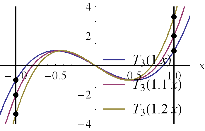
Example: Expand \( \textrm{AF} \) for \( N = 4 \).

The roots of \( T_3(x) \) are

\begin{equation}\label{eqn:chebychevSecondMethod:200}
x_n’ \in \setlr{0, \pm \frac{\sqrt{3}}{2} },
\end{equation}

so the array factor is

\begin{equation}\label{eqn:chebychevSecondMethod:220}
\begin{aligned}
\textrm{AF}
&=
\lr{ z^2 + z \lr{ 2 – \frac{3}{x_0^2} } + 1 }\lr{ z + 1 } \\
&=
z^3
+ 3 z^2 \lr{ 1 – \frac{1}{x_0^2} }
+ 3 z \lr{ 1 – \frac{1}{x_0^2} }
+ 1.
\end{aligned}
\end{equation}

With \( 20 \log_{10} R = 30 \textrm{dB} \), \( x_0 = 2.1 \), so this is

\begin{equation}\label{eqn:chebychevSecondMethod:240}
\textrm{AF} = z^3 + 2.33089 z^2 + 2.33089 z + 1.
\end{equation}

With

\begin{equation}\label{eqn:chebychevSecondMethod:260}
z = e^{j (u + u_0) } = e^{j k d \cos\theta + j k u_0 },
\end{equation}

the array factor takes the form

\begin{equation}\label{eqn:chebychevSecondMethod:280}
\textrm{AF}
=
e^{j 3 k d \cos\theta + j 3 k u_0 }
+ 2.33089
e^{j 2 k d \cos\theta + j 2 k u_0 }
+ 2.33089
e^{j k d \cos\theta + j k u_0 }
+ 1.
\end{equation}

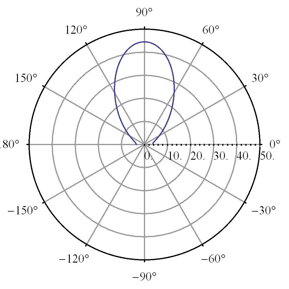
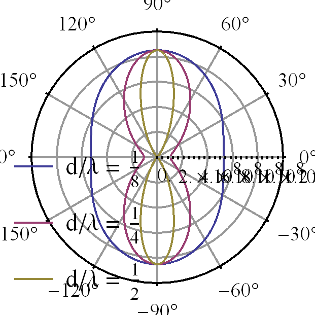
This array function is highly phase dependent, plotted for \( u_0 = 0 \) in fig. 1, and fig. 2.

ChebychevSecondMethodPolarFig3pn

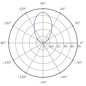
fig 1. Plot with u_0 = 0, d = lambda/4

ChebychevSecondMethodSPolarFig4pn

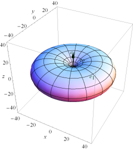
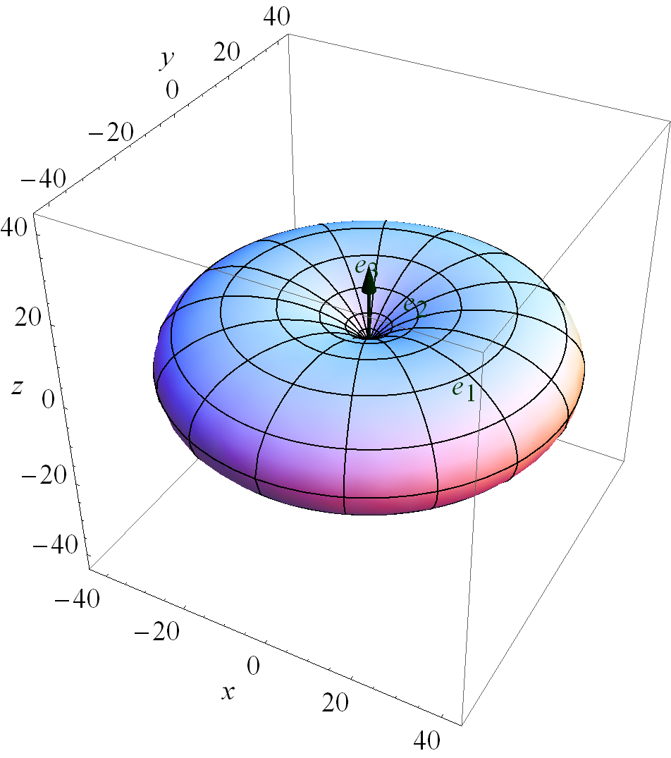
fig 2. Spherical plot with u_0 = 0, d = lambda/4

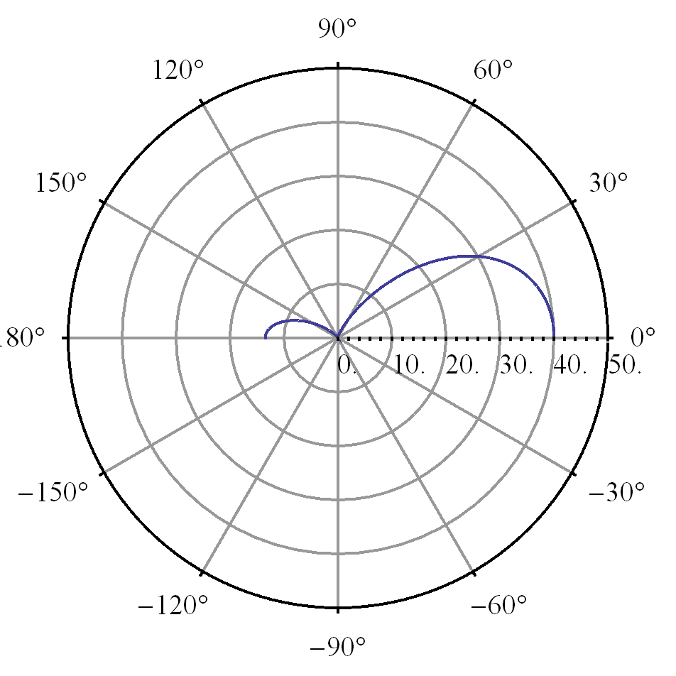
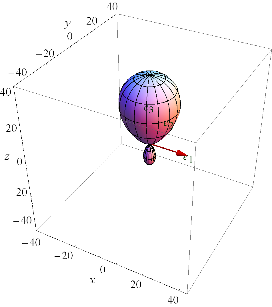
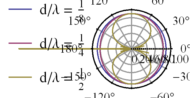
This can be directed along a single direction (z-axis) with higher phase choices as illustrated in fig. 3, and fig. 4.


ChebychevSecondMethodPolarFig1pn

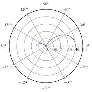
fig 3. Plot with u_0 = 3.5, d = 0.4 lambda

ChebychevSecondMethodSPolarFig2pn

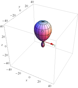
fig 4. Spherical plot with u_0 = 3.5, d = 0.4 lambda


These can be explored interactively in this Mathematica Manipulate panel.

References

[1] Constantine A Balanis. Antenna theory: analysis and design. John Wiley \& Sons, 3rd edition, 2005.

Chebychev antenna array design

March 22, 2015 ece1229 , , , ,

[Click here for a PDF of this post with nicer formatting]

In our text [1] is a design procedure that applies Chebychev polynomials to the selection of current magnitudes for an evenly spaced array of identical antennas placed along the z-axis.

For an even number \( 2 M \) of identical antennas placed at positions \( \Br_m = (d/2) \lr{2 m -1} \Be_3 \), the array factor is

\begin{equation}\label{eqn:chebychevDesign:20}
\textrm{AF}
=
\sum_{m=-N}^N I_m e^{-j k \rcap \cdot \Br_m }.
\end{equation}

Assuming the currents are symmetric \( I_{-m} = I_m \), with \( \rcap = (\sin\theta \cos\phi, \sin\theta \sin\phi, \cos\theta ) \), and \( u = \frac{\pi d}{\lambda} \cos\theta \), this is

\begin{equation}\label{eqn:chebychevDesign:40}
\begin{aligned}
\textrm{AF}
&=
\sum_{m=-N}^N I_m e^{-j k (d/2) ( 2 m -1 )\cos\theta } \\
&=
2 \sum_{m=1}^N I_m \cos\lr{ k (d/2) ( 2 m -1)\cos\theta } \\
&=
2 \sum_{m=1}^N I_m \cos\lr{ (2 m -1) u }.
\end{aligned}
\end{equation}

This is a sum of only odd cosines, and can be expanded as a sum that includes all the odd powers of \( \cos u \). Suppose for example that this is a four element array with \( N = 2 \). In this case the array factor has the form

\begin{equation}\label{eqn:chebychevDesign:60}
\begin{aligned}
\textrm{AF}
&=
2 \lr{ I_1 \cos u + I_2 \lr{ 4 \cos^3 u – 3 \cos u } } \\
&=
2 \lr{ \lr{ I_1 – 3 I_2 } \cos u + 4 I_2 \cos^3 u }.
\end{aligned}
\end{equation}

The design procedure in the text sets \( \cos u = z/z_0 \), and then equates this to \( T_3(z) = 4 z^3 – 3 z \) to determine the current amplitudes \( I_m \). That is

\begin{equation}\label{eqn:chebychevDesign:80}
\frac{ 2 I_1 – 6 I_2 }{z_0} z + \frac{8 I_2}{z_0^3} z^3 = -3 z + 4 z^3,
\end{equation}

or

\begin{equation}\label{eqn:chebychevDesign:100}
\begin{aligned}
\begin{bmatrix}
I_1 \\
I_2
\end{bmatrix}
&=
{\begin{bmatrix}
2/z_0 & -6/z_0 \\
0 & 8/z_0^3
\end{bmatrix}}^{-1}
\begin{bmatrix}
-3 \\
4
\end{bmatrix} \\
&=
\frac{z_0}{2}
\begin{bmatrix}
3 (z_0^2 -1) \\
z_0^2
\end{bmatrix}.
\end{aligned}
\end{equation}

The currents in the array factor are fully determined up to a scale factor, reducing the array factor to

\begin{equation}\label{eqn:chebychevDesign:140}
\textrm{AF} = 4 z_0^3 \cos^3 u – 3 z_0 \cos u.
\end{equation}

The zeros of this array factor are located at the zeros of

\begin{equation}\label{eqn:chebychevDesign:120}
T_3( z_0 \cos u ) = \cos( 3 \cos^{-1} \lr{ z_0 \cos u } ),
\end{equation}

which are at \( 3 \cos^{-1} \lr{ z_0 \cos u } = \pi/2 + m \pi = \pi \lr{ m + \inv{2} } \)

\begin{equation}\label{eqn:chebychevDesign:160}
\cos u = \inv{z_0} \cos\lr{ \frac{\pi}{3} \lr{ m + \inv{2} } } = \setlr{ 0, \pm \frac{\sqrt{3}}{2 z_0} }.
\end{equation}

showing that the scaling factor \( z_0 \) effects the locations of the zeros. It also allows the values at the extremes \( \cos u = \pm 1 \), to increase past the \( \pm 1 \) non-scaled limit values. These effects can be explored in this Mathematica notebook, but can also be seen in fig. 1.

ChebyChevThreeScaledFig2pn

fig 1. T_3( z_0 x) for a few different scale factors z_0.


The scale factor can be fixed for a desired maximum power gain. For \( R
\textrm{dB} \), that will be when

\begin{equation}\label{eqn:chebychevDesign:180}
20 \log_{10} \cosh( 3 \cosh^{-1} z_0 ) = R \textrm{dB},
\end{equation}

or

\begin{equation}\label{eqn:chebychevDesign:200}
z_0 = \cosh \lr{ \inv{3} \cosh^{-1} \lr{ 10^{\frac{R}{20}} } }.
\end{equation}

For \( R = 30 \) dB (say), we have \( z_0 = 2.1 \), and

\begin{equation}\label{eqn:chebychevDesign:220}
\textrm{AF}
= 40 \cos^3 \lr{ \frac{\pi d}{\lambda} \cos\theta } – 6.4 \cos \lr{ \frac{\pi d}{\lambda} \cos\theta }.
\end{equation}

These are plotted in fig. 2 (linear scale), and fig. 3 (dB scale) for a couple values of \( d/\lambda \).

ChebychevT3FittingFig3pn

fig 2. T_3 fitting of 4 element array (linear scale).

ChebychevT3FittingDbFig4pn

fig 3. T_3 fitting of 4 element array (dB scale).

To explore the \( d/\lambda \) dependence try this Mathematica notebook.

References

[1] Constantine A Balanis. Antenna theory: analysis and design. John
Wiley & Sons, 3rd edition, 2005.