[Click here for a PDF of this post with nicer formatting]

Disclaimer

Peeter’s lecture notes from class. These may be incoherent and rough.

These are notes for the UofT course PHY1520, Graduate Quantum Mechanics, taught by Prof. Paramekanti, covering chap 1 (basic concepts),3 (density operator). content from [1].

Basic concepts

We’ve reviewed the basic concepts that we will encounter in Quantum Mechanics.

1. Abstract state vector. \( \ket{ \psi} \)
2. Basis states. \( \ket{ x } \)
3. Observables, special Hermitian operators. We’ll only deal with linear observables.
4. Measurement.

We can either express the wave functions \( \psi(x) = \braket{x}{\psi} \) in terms of a basis for the observable, or can express the observable in terms of the basis of the wave function (position or momentum for example).

We saw that the position space representation of a momentum operator (also an observable) was

\begin{equation}\label{eqn:lecture2:20}
\hat{p} \rightarrow -i \Hbar \PD{x}{}.
\end{equation}

In general we can find the matrix element representation of any operator by considering its representation in a given basis. For example, in a position basis, that would be

\begin{equation}\label{eqn:lecture2:40}
\bra{x’} \hat{A} \ket{x} \leftrightarrow A_{x x’}
\end{equation}

The Hermitian property of the observable means that \( A_{x x’} = A_{x’ x}^\conj \)

\begin{equation}\label{eqn:lecture2:60}
\int dx \bra{x’} \hat{A} \ket{x} \braket{x }{\psi} = \braket{x’}{\phi}
\leftrightarrow
A_{x’ x} \psi_x = \phi_{x’}.
\end{equation}

Example: Measurement example

fig. 1. Polarizer apparatus

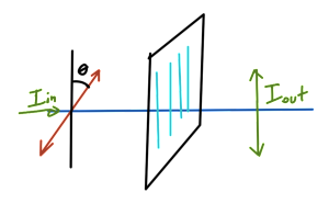
Consider a polarization apparatus as sketched in fig. 1, where the output is of the form \( I_{\textrm{out}} = I_{\textrm{in}} \cos^2 \theta \).

A general input state can be written in terms of each of the possible polarizations

\begin{equation}\label{eqn:lecture2:80}
\alpha \ket{ \updownarrow } + \beta \ket{ \leftrightarrow } \sim
\cos\theta \ket{ \updownarrow } + \sin\theta \ket{ \leftrightarrow }
\end{equation}

Here \( \abs{\alpha}^2 \) is the probability that the input state is in the upwards polarization state, and \( \abs{\beta}^2 \) is the probability that the input state is in the downwards polarization state.

The measurement of the polarization results in an output state that has a specific polarization. That measurement is said to collapse the wavefunction.

When attempting a measurement, looking for a specific value, effects the state of the system, and is call a strong or projective measurement. Such a measurement is

• (i) Probabilistic.
• (ii) Requires many measurements.

This measurement process results a determination of the eigenvalue of the operator. The eigenvalue production of measurement is why we demand that operators be Hermitian.

It is also possible to try to do a weaker (perturbative) measurement, where some information is extracted from the input state without completely altering it.

Time evolution

1. Schrodinger picture.
   The time evolution process is governed by a Schrodinger equation of the following form\begin{equation}\label{eqn:lecture2:100}
   i \Hbar \PD{t}{} \ket{\Psi(t)} = \hat{H} \ket{\Psi(t)}.
   \end{equation}

   This Hamiltonian could be, for example,

   \begin{equation}\label{eqn:lecture2:120}
   \hat{H} = \frac{\hat{p}^2}{2m} + V(x),
   \end{equation}

   Such a representation of time evolution is expressed in terms of operators \( \hat{x}, \hat{p}, \hat{H}, \cdots \) that are independent of time.

2. Heisenberg picture.Suppose we have a state \( \ket{\Psi(t)} \) and operate on this with an operator

   \begin{equation}\label{eqn:lecture2:140}
   \hat{A} \ket{\Psi(t)}.
   \end{equation}

   This will have time evolution of the form

   \begin{equation}\label{eqn:lecture2:160}
   \hat{A} e^{-i \hat{H} t/\Hbar} \ket{\Psi(0)},
   \end{equation}

   or in matrix element form

   \begin{equation}\label{eqn:lecture2:180}
   \bra{\phi(t)} \hat{A} \ket{\Psi(t)}
   =
   \bra{\phi(0)}
   e^{i \hat{H} t/\Hbar}
   \hat{A} e^{-i \hat{H} t/\Hbar} \ket{\Psi(0)}.
   \end{equation}

   We work with states that do not evolve in time \( \ket{\phi(0)}, \ket{\Psi(0)}, \cdots \), but operators do evolve in time according to

   \begin{equation}\label{eqn:lecture2:200}
   \hat{A}(t) =
   e^{i \hat{H} t/\Hbar}
   \hat{A} e^{-i \hat{H} t/\Hbar}.
   \end{equation}

Density operator

We can have situations where it is impossible to determine a single state that describes the system. For example, given the gas in the room that you are sitting in, there are things that we can measure, but it is impossible to describe the state that describes all the particles and also impossible to construct a Hamiltonian that governs all the interactions of those many many particles.

We need a probabilistic description to even describe such a complex system.

Suppose we have a complex system that can be partitioned into two subsets, left and right, as sketched in fig. 2.

fig. 2. System partitioned into separate set of states

If the states in each partition can be enumerated separately, we can write the state of the system as sums over the probability amplitudes that for the combined states.

\begin{equation}\label{eqn:lecture2:220}
\ket{\Psi}
=
\sum_{m, n} C_{m,n} \ket{m} \ket{n}
\end{equation}

Here \( C_{m, n} \) is the probability amplitude to find the state in the combined state \( \ket{m} \ket{n} \).

As an example of such a system, we could investigate a two particle configuration where spin up or spin down can be separately measured for each particle.

\begin{equation}\label{eqn:lecture2:240}
\ket{\psi} = \inv{\sqrt{2}} \lr{
\ket{\uparrow}\ket{\downarrow}
+
\ket{\downarrow}\ket{\rightarrow}
}
\end{equation}

Considering such a system we could ask questions such as

• What is the probability that the left half is in state \( m \)? This would be\begin{equation}\label{eqn:lecture2:260}
  \sum_n \Abs{C_{m, n}}^2
  \end{equation}
• Probability that the left half is in state \( m \), and the
  probability that the right half is in state \( n \)? That is\begin{equation}\label{eqn:lecture2:280}
  \Abs{C_{m, n}}^2
  \end{equation}

We define the density operator

\begin{equation}\label{eqn:lecture2:300}
\hat{\rho} = \ket{\Psi} \bra{\Psi}.
\end{equation}

This is idempotent

\begin{equation}\label{eqn:lecture2:320}
\hat{\rho}^2 =
\lr{ \ket{\Psi} \bra{\Psi} }
\lr{ \ket{\Psi} \bra{\Psi} }
=
\ket{\Psi} \bra{\Psi}
\end{equation}

References

[1] Jun John Sakurai and Jim J Napolitano. Modern quantum mechanics. Pearson Higher Ed, 2014.