[Click here for a PDF of this post with nicer formatting]
Both [3] and [4] use Gaussian integrals with both (negative) real, and imaginary arguments, which give the impression that the following is true:
\begin{equation}\label{eqn:generalizedGaussian:20}
\int_{-\infty}^\infty \exp\lr{ a x^2 } dx = \sqrt{\frac{-\pi}{a}},
\end{equation}
even when \( a \) is not a real negative constant, and in particular, with values \( a = \pm i \). Clearly this doesn’t follow by just making a substition \( x \rightarrow x/\sqrt{a} \), since that moves the integration range onto a rotated path in the complex plane when \( a \) is \( \pm i \). However, with some care, it can be shown that \ref{eqn:generalizedGaussian:20} holds provided \( \textrm{Re} \, a \le 0 \).
The first special case is \( \int_{-\infty}^\infty \exp\lr{ – x^2 } dx = \sqrt{\pi} \) which is easy to derive using the usual square it and integrate in circular coordinates trick.
Purely imaginary cases.
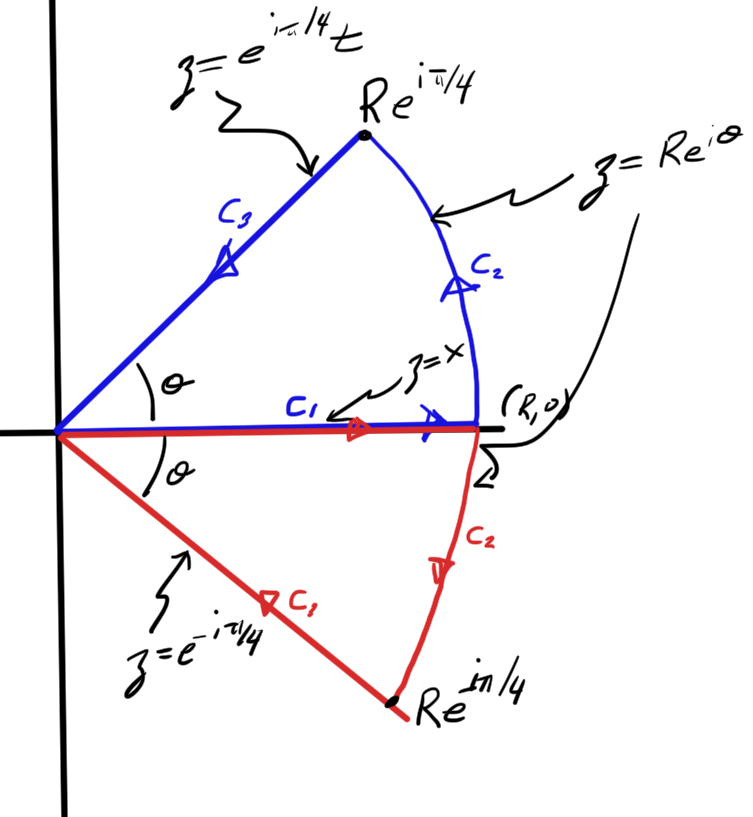
Let’s handle the \( a = \pm i \) cases next. These can be evaluated by considering integrals over the contours of fig. 1, where the upper plane contour is used for \( a = i \) and the lower plane contour for \( a = -i \).
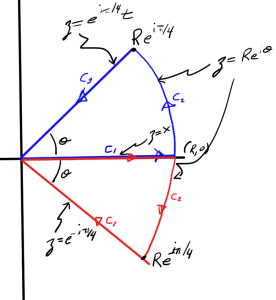
fig. 1. Contours for a = i,-i
Since there are no poles, the integral over either such contour is zero. Credit for figuring out how to tackle that integral and what contour to use goes to Dr MV, on stackexchange [2].
For the upper plane contour we have
\begin{equation}\label{eqn:generalizedGaussian:40}
\begin{aligned}
0
&= \oint \exp\lr{ i z^2 } dz \\
&= \int_0^R \exp\lr{ i x^2 } dx
+ \int_0^{\pi/4} \exp\lr{ i R^2 e^{2 i \theta} } R i e^{i\theta} d\theta
+ \int_R^0 \exp\lr{ i^2 t^2 } e^{i\pi/4} dt.
\end{aligned}
\end{equation}
Observe that \( i e^{2 i \theta} = i\cos(2 \theta) – \sin(2\theta) \) which has a negative real part for all values of \( \theta \ne 0 \). Provided the contour is slightly deformed from the axis, that second integral has a term of the form \( \sim R e^{-R^2} \) which tends to zero as \( R \rightarrow \infty \). So in the limit, this is
\begin{equation}\label{eqn:generalizedGaussian:60}
\int_0^\infty \exp\lr{ i x^2 } dx
= \sqrt{\pi} e^{i\pi/4}/2,
\end{equation}
or
\begin{equation}\label{eqn:generalizedGaussian:80}
\int_{-\infty}^\infty \exp\lr{ i x^2 } dx
= \sqrt{i \pi},
\end{equation}
a special case of \ref{eqn:generalizedGaussian:20} as desired. For \( a = -i \) integrating around the lower plane contour, we have
\begin{equation}\label{eqn:generalizedGaussian:100}
\begin{aligned}
0
&= \oint \exp\lr{ -i z^2 } dz \\
&= \int_0^R \exp\lr{ i x^2 } dx
+ \int_0^{-\pi/4} \exp\lr{ -i R^2 e^{2 i \theta} } R i e^{i\theta} d\theta
+ \int_R^0 \exp\lr{ -i (-i) t^2 } e^{-i\pi/4} dt.
\end{aligned}
\end{equation}
This time, in the second integral we also have \( -i R^2 e^{2 i \theta} = i R^2 \cos(2 \theta) + \sin(2 \theta) \), which also has a negative real part for \( \theta \in (0, \pi/4] \). Again the contour needs to be infinitesimally deformed, placed just lower than the axis.
This time we find
\begin{equation}\label{eqn:generalizedGaussian:120}
\int_{-\infty}^\infty \exp\lr{ -i x^2 } dx
= \sqrt{-i \pi},
\end{equation}
another special case of \ref{eqn:generalizedGaussian:20}.
Note.
Distorting the contour in this fashion seems somewhat like handwaving. A better approach would probably follow [1] where Jordan’s lemma is covered. It doesn’t look like Jordan’s lemma applies as is to this case, but the arguments look like they could be adapted appropriately.
Completely complex case.
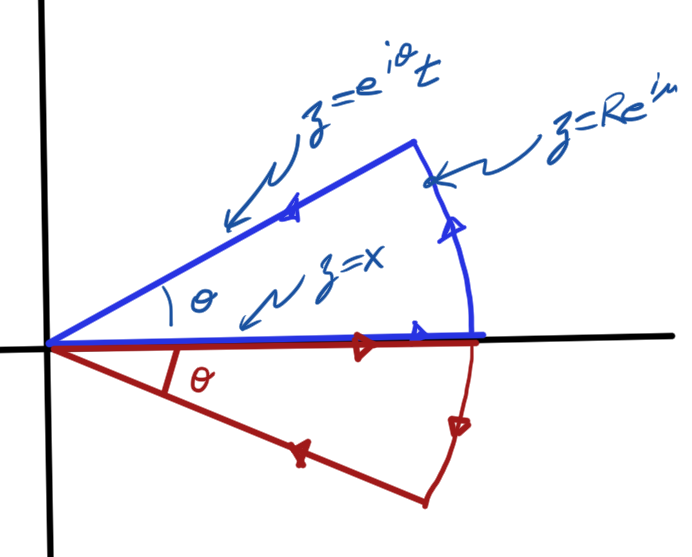
A similar trick can be used to evaluate the more general cases, but a bit of thought is required to figure out the contours required. More precisely, while these contours will still have a wedge of pie shape, as sketched in fig. 2, we have to figure out the angle subtended by the edge of this piece of pie.
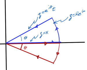
fig. 2. Contours for complex a.
To evaluate an integral consider
\begin{equation}\label{eqn:generalizedGaussian:140}
\begin{aligned}
0
&= \oint \exp\lr{ e^{i\phi} z^2 } dz \\
&= \int_0^R \exp\lr{ e^{i\phi} x^2 } dx
+ \int_0^{\theta} \exp\lr{ e^{i\phi} R^2 e^{2 i \mu} } R i e^{i\mu} d\mu
+ \int_R^0 \exp\lr{ e^{i\phi} e^{2 i \theta} t^2 } e^{i\theta} dt,
\end{aligned}
\end{equation}
where \( \phi \in (\pi/2, \pi) \cup (\pi,3\pi/2) \). We have a hope of evaluating this last integral if \( \phi + 2 \theta = \pi \), or
\begin{equation}\label{eqn:generalizedGaussian:160}
\theta = (\pi -\phi)/2,
\end{equation}
giving
\begin{equation}\label{eqn:generalizedGaussian:180}
\int_0^R \exp\lr{ e^{i\phi} x^2 } dx
=
e^{i\lr{\pi – \phi}/2} \int_0^R \exp\lr{ -t^2 } dt
– \int_0^{\theta} \exp\lr{ R^2 \lr{ \cos\lr{\phi + 2 \mu} + i \sin\lr{\phi + 2 \mu}} } R i e^{i\mu} d\mu.
\end{equation}
If the cosine is always negative on the chosen contours, then that integral will vanish in the \( R \rightarrow \infty \) limit. This turns out to be the case, which can be confirmed by considering each of the contours in sequence. If the upper plane contour is used to evaluate the integral for the \( \phi \in (\pi/2,\pi) \) case, we have
\begin{equation}\label{eqn:generalizedGaussian:200}
\theta \in (0, \pi/4).
\end{equation}
Since \( \phi + 2\theta = \pi \), we have
\begin{equation}\label{eqn:generalizedGaussian:220}
\phi + 2 \mu \in (\pi/2, \pi),
\end{equation}
and find that the cosine is strictly negative on that contour for that range of \( \phi \). Picking the lower plane contour for the \( \phi \in (\pi, 3\pi/2) \) range, we have
\begin{equation}\label{eqn:generalizedGaussian:240}
\theta \in (-\pi/4, 0),
\end{equation}
and so
\begin{equation}\label{eqn:generalizedGaussian:260}
\phi + 2 \mu \in (\pi/2, 3\pi/2).
\end{equation}
For this range of \( \phi \) the cosine on the lower plane contour is again negative as desired, so in the infinite \( R \) limit we have
\begin{equation}\label{eqn:generalizedGaussian:280}
\int_0^\infty \exp\lr{ e^{i\phi} x^2 } dx
=
\inv{2} \sqrt{ -\pi e^{-i\phi} }.
\end{equation}
The points at \( \phi = \pi/2, \pi, 3\pi/2 \) were omitted, but we’ve found the same result at those points, completing the verification of \ref{eqn:generalizedGaussian:20} for all \( \textrm{Re} a \le 0 \).
References
[1] W.R. Le Page and W.R. LePage. Complex Variables and the Laplace Transform for Engineers, chapter 8-10. A Theorem for Trigonometric Integrals. Courier Dover Publications, 1980.
[2] Dr. MV. Evaluating definite integral of exp(i t^2), 2015. URL https://math.stackexchange.com/a/1411084/359. [Online; accessed 10-September-2015].
[3] Jun John Sakurai and Jim J Napolitano. Modern quantum mechanics. Pearson Higher Ed, 2014.
[4] A. Zee. Quantum field theory in a nutshell. Universities Press, 2005.