[Click here for a PDF of this post with nicer formatting]
Motivation
Check out fig. 1, a handout given to my daughter has a handout from her grade 11 physics class, titled “The Big Five”, covering some dynamics equations.
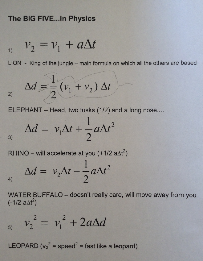
fig. 1. The Big Five… in Physics
I found this handout disorienting. Part of that disorientation is because of the weird African animal theme which I couldn’t see the rationale for. Aurora showed me that the second equation can be outlined with an elephant, apparently justifying the animal theme. The equations themselves are not in a form that I would have expected, and have a lot of redundancy built in. The assumptions required for these equations to be valid are also not stated. Those equations are
\begin{equation}\label{eqn:theBigFivePhysics:40}
v_2 = v_1 + a \Delta t
\end{equation}
\begin{equation}\label{eqn:theBigFivePhysics:60}
\Delta d = \inv{2} \lr{ v_1 + v_2 } \Delta t
\end{equation}
\begin{equation}\label{eqn:theBigFivePhysics:80}
\Delta d = v_1 \Delta t + \inv{2} a \lr{\Delta t}^2
\end{equation}
\begin{equation}\label{eqn:theBigFivePhysics:100}
\Delta d = v_2 \Delta t – \inv{2} a \lr{\Delta t}^2
\end{equation}
\begin{equation}\label{eqn:theBigFivePhysics:120}
v_2^2 = v_1^2 + 2 a \Delta d.
\end{equation}
Reverse engineering “the big five”.
Difference of velocity
The first equation \ref{eqn:theBigFivePhysics:40} is just a discrete version of the definition of scalar acceleration
\begin{equation}\label{eqn:theBigFivePhysics:140}
a = \frac{dv}{dt}.
\end{equation}
The approximation of that is
\begin{equation}\label{eqn:theBigFivePhysics:160}
a = \frac{\Delta v}{\Delta t},
\end{equation}
or
\begin{equation}\label{eqn:theBigFivePhysics:180}
\Delta v = v_2 – v_1 = a \Delta t.
\end{equation}
Constant acceleration
Next in the list, it’s clear that the equation(s) for \( \Delta d \) is really based on an assumption of constant acceleration. In fact, all four of the next equations are nothing more than variations of
\begin{equation}\label{eqn:theBigFivePhysics:200}
v = a t.
\end{equation}
To arrive at fig. 2.

fig. 2. Displacement as area under the curve.
Should we wish to integrate, it’s the second simplest integral we could possibly do
\begin{equation}\label{eqn:theBigFivePhysics:220}
\begin{aligned}
\Delta x
&= \int_{t_1}^{t_2} v(t) dt \\
&= \int_{t_1}^{t_2} a t dt \\
&= \inv{2} a \lr{ t_2^2 – t_1^2 } \\
&= \inv{2} a \Delta t \lr{ t_2 + t_1 }.
\end{aligned}
\end{equation}
This looks a little different than what’s on the formula cheet, but since (for constant acceleration) we have
\begin{equation}\label{eqn:theBigFivePhysics:240}
t = \frac{v}{a},
\end{equation}
this can be written as
\begin{equation}\label{eqn:theBigFivePhysics:260}
\begin{aligned}
\Delta x
&= \inv{2} a \Delta t \lr{ \frac{v_2}{a} + \frac{v_1}{a} } \\
&= \inv{2} \Delta t \lr{ v_1 + v_2 },
\end{aligned}
\end{equation}
as found on the formula sheet (except for them using \( \Delta d \) for the difference in position .)
Each of the next equations follow from straight algebra
\begin{equation}\label{eqn:theBigFivePhysics:280}
\begin{aligned}
\Delta x – v_1 \Delta t
&= \inv{2} \Delta t \lr{ v_1 + v_2 } – v_1 \Delta t \\
&= \inv{2} \Delta t \lr{ -v_1 + v_2 } \\
&= \inv{2} \lr{\Delta t}^2 \frac{\Delta v}{\Delta t} \\
&= \inv{2} a \lr{\Delta t}^2,
\end{aligned}
\end{equation}
and
\begin{equation}\label{eqn:theBigFivePhysics:300}
\begin{aligned}
\Delta x – v_2 \Delta t
&= \inv{2} \Delta t \lr{ v_1 + v_2 } – v_2 \Delta t \\
&= \inv{2} \Delta t \lr{ v_1 – v_2 } \\
&= -\inv{2} \lr{\Delta t}^2 \frac{\Delta v}{\Delta t} \\
&= -\inv{2} a \lr{\Delta t}^2,
\end{aligned}
\end{equation}
and finally
\begin{equation}\label{eqn:theBigFivePhysics:320}
\begin{aligned}
\Delta x
&= \inv{2} a \lr{ t_2^2 – t_1^2 } \\
&= \inv{2 a } \lr{ v_2^2 – v_1^2 }.
\end{aligned}
\end{equation}
A better set of equations.
If I had to write these “big five” equation, I’d be more inclined to write them as
\begin{equation}\label{eqn:theBigFivePhysics:360}
a = \frac{\Delta v}{\Delta t}
\end{equation}
\begin{equation}\label{eqn:theBigFivePhysics:380}
v = a t = \frac{\Delta x}{\Delta t}
\end{equation}
\begin{equation}\label{eqn:theBigFivePhysics:400}
\Delta x = \int_{t_1}^{t_2} v dt = \inv{2} a \lr{ t_2^2 – t_1^2 }
\end{equation}
\begin{equation}\label{eqn:theBigFivePhysics:420}
t_1 = \frac{v_1}{a}
\end{equation}
\begin{equation}\label{eqn:theBigFivePhysics:440}
t_2 = \frac{v_2}{a}.
\end{equation}
Anything more than that is just algebra. The last two could be omitted since they really follow from \ref{eqn:theBigFivePhysics:380}. For high school where calculus isn’t known, I’d swap out \ref{eqn:theBigFivePhysics:400} for \ref{eqn:theBigFivePhysics:60} which can be derived graphically by understanding that the distance is the area under the velocity curve.
I’d also leave out all mentions of big African animals, which is, just plain weird!