[Click here for a PDF of this post with nicer formatting]
DISCLAIMER: Very rough notes from class, with some additional side notes.
These are notes for the UofT course PHY2403H, Quantum Field Theory I, taught by Prof. Erich Poppitz fall 2018.
Lorentz transform symmetries.
From last time, recall that an infinitesimal Lorentz transform has the form
\begin{equation}\label{eqn:qftLecture10:20}
x^\mu \rightarrow x^\mu + \omega^{\mu\nu} x_\nu,
\end{equation}
where
\begin{equation}\label{eqn:qftLecture10:40}
\omega^{\mu\nu} = -\omega^{\nu\mu}
\end{equation}
We showed last time that \( \omega^{ij} \) induces a rotation, and will show today that \( \omega^{0i} \) is a boost.
We introduced a three index current, factoring out explicit dependence on the incremental Lorentz transform tensor \( \omega^{\mu\nu} \) as follows
\begin{equation}\label{eqn:qftLecture10:80}
J^{\nu \mu\rho} = \inv{2} \lr{ x^\rho T^{\nu\mu} – x^\mu T^{\nu\rho} },
\end{equation}
and can easily show that this current has the desired zero four-divergence property
\begin{equation}\label{eqn:qftLecture10:100}
\begin{aligned}
\partial_\nu J^{\nu \mu\rho}
&= \inv{2} \lr{
(\partial_\nu x^\rho) T^{\nu\mu}
+
x^\rho {\partial_\nu T^{\nu\mu} }
– (\partial_\nu x^\mu) T^{\nu\rho}
– x^\mu {\partial_\nu T^{\nu\rho} }
} \\
&= \inv{2} \lr{
(\partial_\nu x^\rho) T^{\nu\mu}
– (\partial_\nu x^\mu) T^{\nu\rho}
} \\
&= \inv{2} \lr{
T^{\rho\mu}
+
– T^{\mu\rho}
} \\
&= 0,
\end{aligned}
\end{equation}
since the energy-momentum tensor is symmetric.
Defining charge in the usual fashion \( Q = \int d^3 x j^0 \), so we can define a charge for each pair of indexes \( \mu\nu \), and in particular
\begin{equation}\label{eqn:qftLecture10:120}
Q^{0k} = \int d^3 x J^{0 0 k} = \inv{2} \int d^3 x \lr{ x^k T^{00} – x^0 T^{0k} }
\end{equation}
\begin{equation}\label{eqn:qftLecture10:540}
\begin{aligned}
\dot{Q}^{0k}
&= \int d^3 x \dot{J}^{0 0k} \\
&= \inv{2} \int d^3 x \lr{ x^k \dot{T}^{00} – x^0 \dot{T}^{0k} }
\end{aligned}
\end{equation}
However, since \( 0 = \partial_\mu T^{\mu \nu} = \dot{T}^{0 \nu} + \partial_j T^{j \nu} \), or \( \dot{T}^{0 \nu} = -\partial_j T^{j \nu} \),
\begin{equation}\label{eqn:qftLecture10:560}
\begin{aligned}
\dot{Q}^{0k}
&= \inv{2} \int d^3 x \lr{ x^k (-\partial_j T^{j0}) – T^{0k} – x^0 (-\partial_j T^{jk}) } \\
&= \inv{2} \int d^3 x \lr{
\partial_j (-x^k T^{j0}) + (\partial_j x^k) T^{j0}
– T^{0k} + x^0 \partial_j T^{jk}
} \\
&= \inv{2} \int d^3 x \lr{
\partial_j (-x^k T^{j0}) + {T^{k0}}
– {T^{0k}} + x^0 \partial_j T^{jk}
} \\
&= \inv{2} \int d^3 x \lr{
\partial_j (-x^k T^{j0})
+ x^0 \partial_j T^{jk}
} \\
&= \inv{2} \int d^3 x
\partial_j \lr{
-x^k T^{j0}
+ x^0 T^{jk}
},
\end{aligned}
\end{equation}
which leaves just surface terms, so \( \dot{Q}^{0k} = 0 \).
Quantizing:
From our previous identification
\begin{equation}\label{eqn:qftLecture9:560}
–
{T^\nu}_\mu =
-\partial^\nu \phi \partial_\mu \phi + {\delta^{\nu}}_\mu \LL,
\end{equation}
we have
\begin{equation}\label{eqn:qftLecture10:580}
T^{\nu\mu} = \partial^\nu \phi \partial^\mu \phi – g^{\nu\mu} \LL,
\end{equation}
or
\begin{equation}\label{eqn:qftLecture10:600}
\begin{aligned}
T^{00}
&= \partial^0 \phi \partial^0 \phi – \inv{2} \lr{ \partial_0 \phi \partial^0 \phi + \partial_k \phi \partial^k \phi } \\
&= \inv{2} \partial^0 \phi \partial^0 \phi – \inv{2} (\spacegrad \phi)^2,
\end{aligned}
\end{equation}
and
\begin{equation}\label{eqn:qftLecture10:620}
T^{0k} = \partial^0 \phi \partial^k \phi,
\end{equation}
so we may quantize these energy momentum tensor components as
\begin{equation}\label{eqn:qftLecture10:640}
\begin{aligned}
\hatT^{00} &= \inv{2} \hat{\pi}^2 + \inv{2} (\spacegrad \phihat)^2 \\
\hatT^{0k} &= \inv{2} \hat{\pi} \partial^k \phihat.
\end{aligned}
\end{equation}
We can now start computing the commutators associated with the charge operator. The first of those commutators is
\begin{equation}\label{eqn:qftLecture10:140}
\antisymmetric{\hatT^{00}(\Bx)}{\phihat(\By)}
=
\inv{2}
\antisymmetric{\hat{\pi}^2(\Bx)}{\phihat(\By)},
\end{equation}
which can be evaluated using the field commutator analogue of \( \antisymmetric{F(p)}{q} = i F’ \) which is
\begin{equation}\label{eqn:qftLecture10:660}
\antisymmetric{F(\hat{\pi}(\Bx))}{\phihat(\By)} = -i \frac{dF}{d \hat{\pi}} \delta(\Bx – \By),
\end{equation}
to give
\begin{equation}\label{eqn:qftLecture10:680}
\antisymmetric{\hatT^{00}(\Bx)}{\phihat(\By)}
= -i \delta^3(\Bx – \By) \hat{\pi}(\Bx)
\end{equation}
The other required commutator is
\begin{equation}\label{eqn:qftLecture10:160}
\begin{aligned}
\antisymmetric{\hatT^{0i}(\Bx)}{\phihat(\By)}
&=
\antisymmetric{\hat{\pi}(\Bx)\partial^i \phihat(\Bx)}{\phihat(\By)} \\
&=
\partial^i \phihat(\Bx)
\antisymmetric{\hat{\pi}(\Bx)
}{\phihat(\By)} \\
&= -i \delta^3(\Bx – \By) \partial^i \phihat(\Bx),
\end{aligned}
\end{equation}
The charge commutator with the field can now be computed
\begin{equation}\label{eqn:qftLecture10:180}
\begin{aligned}
i \epsilon \antisymmetric{\hatQ^{0k}}{\phihat(\By)}
&=
i
\frac{\epsilon}{2} \int d^3 x
\lr{
x^k
\antisymmetric{\hatT^{00}}{\phihat(\By)}
–
x^0
\antisymmetric{\hatT^{0k}}{\phihat(\By)}
} \\
&=
\frac{\epsilon}{2} \lr{ y^k \hat{\pi}(\By) – y^0 \partial^k \phihat(\By) } \\
&=
\frac{\epsilon}{2} \lr{ y^k \dot{\phihat}(\By) – y^0 \partial^k \phihat(\By) },
\end{aligned}
\end{equation}
so to first order in \( \epsilon \)
\begin{equation}\label{eqn:qftLecture10:200}
e^{i \epsilon \hatQ^{0k} } \phihat(\By)
e^{-i \epsilon \hatQ^{0k} }
=
\phihat(\By)
+ \frac{\epsilon}{2} y^k \dot{\phihat}(\By)
+ \frac{\epsilon}{2} y^0 \partial_k \phihat(\By)
\end{equation}
For example, with \( k = 1 \)
\begin{equation}\label{eqn:qftLecture10:700}
\begin{aligned}
e^{i \epsilon \hatQ^{0k} } \phihat(\By)
e^{-i \epsilon \hatQ^{0k} }
&=
\phihat(\By)
+ \frac{\epsilon}{2} \lr{
y^1 \dot{\phihat}(\By)
+
y^0 \PD{y^1}{\phihat}(\By)
} \\
&=
\phihat(y^0 + \frac{\epsilon}{2} y^1,
y^1 + \frac{\epsilon}{2} y^2, y^3).
\end{aligned}
\end{equation}
This is a boost. If we compare explicitly to an infinitesimal Lorentz transformation of the coordinates
\begin{equation}\label{eqn:qftLecture10:220}
\begin{aligned}
x^0 \rightarrow x^0 + \omega^{01} x_1 &= x^0 – \omega^{01} x^1 \\
x^1 \rightarrow x^1 + \omega^{10} x_0 &= x^1 – \omega^{01} x_0 = x^1 – \omega^{01} x^0
\end{aligned}
\end{equation}
we can make the identification
\begin{equation}\label{eqn:qftLecture10:240}
\frac{\epsilon}{2} = – \omega^{01}.
\end{equation}
We now have the explicit form of the generator of a spacetime translation
\begin{equation}\label{eqn:qftLecture10:260}
\boxed{
\hatU(\Lambda) = \exp\lr{-i \omega^{0k} \int d^3 x \lr{ \hatT^{00} x^k – \hatT^{0k} x^0 }}
}
\end{equation}
An explicit boost along the x-axis has the form
\begin{equation}\label{eqn:qftLecture10:300}
\hatU(\Lambda) \phihat(t, \Bx)
\hatU^\dagger(\Lambda)
=
\phihat\lr{ \frac{t – vx}{\sqrt{1 – v^2}}, \frac{x – vt}{\sqrt{1 – v^2}}, y, z },
\end{equation}
and more generally
\begin{equation}\label{eqn:qftLecture10:320}
\hatU(\Lambda) \phihat(x) \hatU^\dagger(\Lambda) =
\phihat(\Lambda x)
\end{equation}
where \( x \) is a four vector, \( (\Lambda x)^\mu = {{\Lambda}^\mu}_\nu x^\nu \), and \(
{{\Lambda}^\mu}_\nu
\approx
{{\delta}^\mu}_\nu
+
{{\omega}^\mu}_\nu \).
Transformation of momentum states
In the momentum space representation
\begin{equation}\label{eqn:qftLecture10:340}
\begin{aligned}
\phihat(x)
&=
\int \frac{d^3 p}{(2 \pi)^3 \sqrt{2 \omega_\Bp}} \lr{
e^{i (\omega_\Bp t – \Bp \cdot \Bx)} \hat{a}_\Bp
+
e^{-i (\omega_\Bp t – \Bp \cdot \Bx)} \hat{a}^\dagger_\Bp
} \\
&=
\int \frac{d^3 p}{(2 \pi)^3 \sqrt{2 \omega_\Bp}} \evalbar{
\lr{
e^{i p^\mu x^\mu } \hat{a}_\Bp
+
e^{-i p^\mu x^\mu } \hat{a}^\dagger_\Bp
}
}{p_0 = \omega_\Bp}
\end{aligned}
\end{equation}
\begin{equation}\label{eqn:qftLecture10:720}
\begin{aligned}
\hatU(\Lambda) \phihat(x) \hatU^\dagger(\Lambda)
&=
\phihat(\Lambda x) \\
&=
\int \frac{d^3 p}{(2 \pi)^3 \sqrt{2 \omega_\Bp}} \evalbar{
\lr{
e^{i p^\mu {{\Lambda}^\mu}_\nu x^\nu }
\hat{a}_\Bp
+
e^{-i p^\mu {{\Lambda}^\mu}_\nu x^\nu } \hat{a}^\dagger_\Bp
}
}{p_0 = \omega_\Bp}
\end{aligned}
\end{equation}
This can be put into an explicitly Lorentz invariant form
\begin{equation}\label{eqn:qftLecture10:n}
\begin{aligned}
\phihat(\Lambda x)
&=
\int \frac{dp^0 d^3 p}{(2\pi)^3} \delta(p_0^2 – \Bp^2 – m^2) \Theta(p^0) \sqrt{2 \omega_\Bp}
e^{i p^\mu {{\Lambda}^\mu}_\nu x^\nu }
\hat{a}_\Bp + \text{h.c.} \\
&=
\int \frac{dp^0 d^3 p}{(2\pi)^3}
\lr{
\frac{\delta(p_0 – \omega_\Bp)}{2 \omega_\Bp}
+
\frac{\delta(p_0 + \omega_\Bp)}{2 \omega_\Bp}
}
\Theta(p^0) \sqrt{2 \omega_\Bp} \hat{a}_\Bp + \text{h.c.},
\end{aligned}
\end{equation}
which recovers \ref{eqn:qftLecture10:720} by making use of the delta function identity \( \delta(f(x)) = \sum_{f(x_\conj) = 0} \frac{\delta(x – x_\conj)}{f'(x_\conj)} \), since the \( \Theta(p^0) \) kills the second delta function.
We now have a more explicit Lorentz invariant structure
\begin{equation}\label{eqn:qftLecture10:380}
\phihat(\Lambda x)
=
\int \frac{dp^0 d^3 p}{(2\pi)^3} \delta(p_0^2 – \Bp^2 – m^2) \Theta(p^0) \sqrt{2 \omega_\Bp}
e^{i p^\mu {{\Lambda}^\mu}_\nu x^\nu }
\hat{a}_\Bp + \text{h.c.}
\end{equation}
Recall that a boost moves a spacetime point along a parabola, such as that of fig. 1, whereas a rotation moves along a constant “circular” trajectory of a hyper-paraboloid. In general, a Lorentz transformation may move a spacetime point along any path on a hyper-paraboloid such as the one depicted (in two spatial dimensions) in fig. 2. This paraboloid depict the surfaces of constant energy-momentum \( p^0 = \sqrt{ \Bp^2 + m^2 } \). Because a Lorentz transformation only shift points along that energy-momentum surface, but cannot change the sign of the energy coordinate \( p^0 \), this means that \( \Theta(p^0) \) is also a Lorentz invariant.
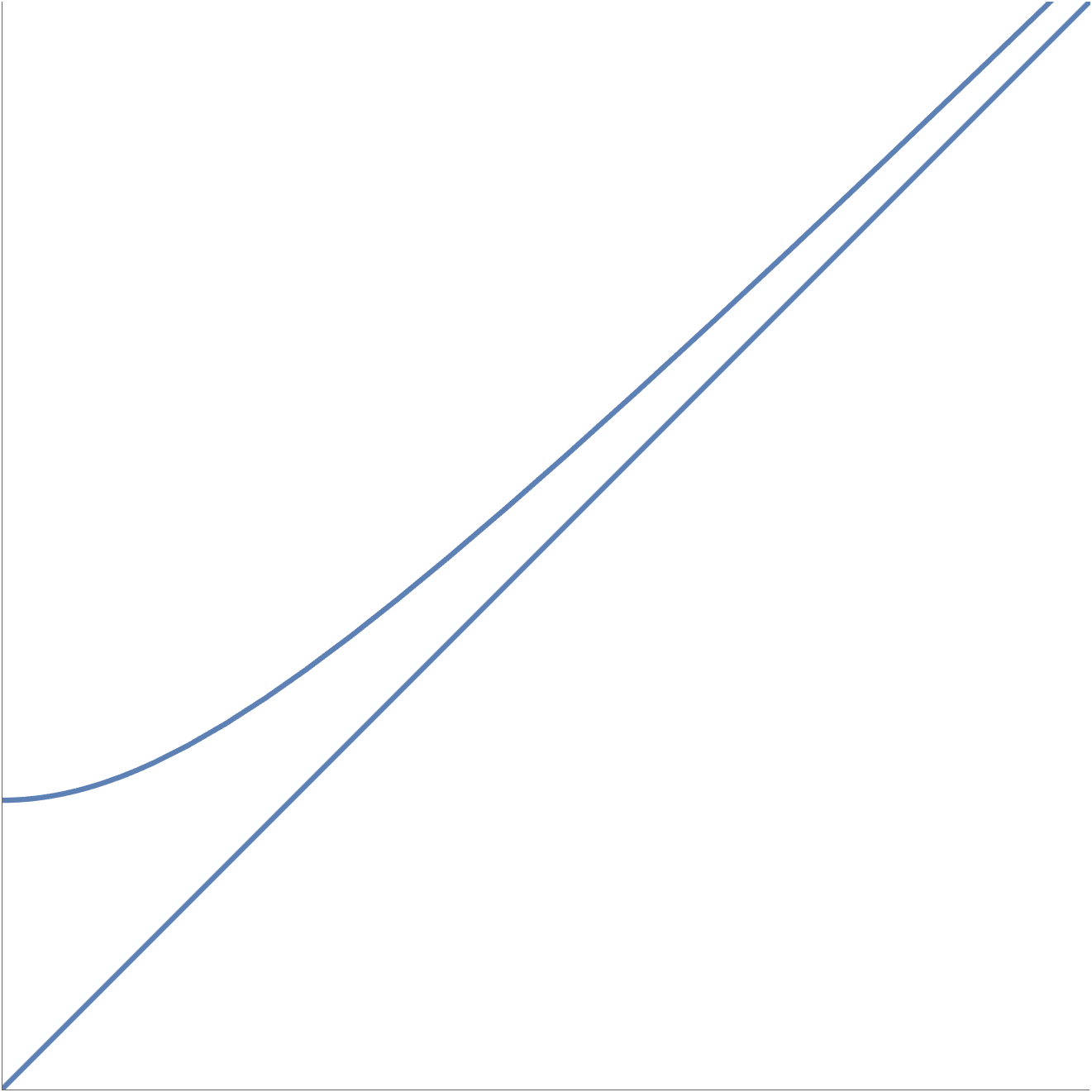
fig. 1. One dimensional spacetime surface for constant (p^0)^2 – p^2 = m^2.
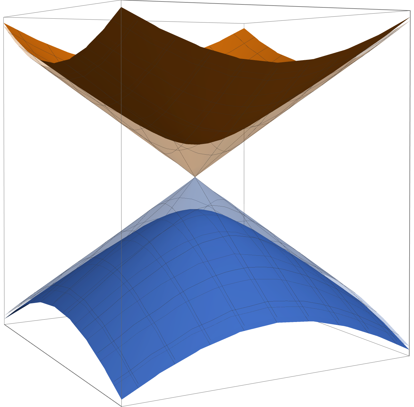
fig. 2. Surface of constant squared four-momentum.
Let’s change variables
\begin{equation}\label{eqn:qftLecture10:400}
p^\lambda = {{\Lambda}^\lambda}_\rho {p’}^{\rho}
\end{equation}
so that
\begin{equation}\label{eqn:qftLecture10:420}
\begin{aligned}
p_\mu
{{\Lambda}^\mu}_\nu x^\nu
&=
{{\Lambda}^\lambda}_\rho {p’}^\rho g_{\lambda\nu} {{\Lambda}^\nu}_\sigma x^{\sigma} \\
&=
{p’}^\rho
\lr{ {{\Lambda}^\lambda}_\rho
g_{\lambda\nu} {{\Lambda}^\nu}_\sigma } x^{\sigma} \\
&=
{p’}^\rho g_{\rho\sigma} x^\sigma
\end{aligned}
\end{equation}
which gives
\begin{equation}\label{eqn:qftLecture10:440}
\begin{aligned}
\phihat(\Lambda x)
&=
\int \frac{d{p’}^0 d^3 p’}{(2\pi)^3} \delta({p’}_0^2 – {\Bp’}^2 – m^2) \Theta(p^0) \sqrt{2 \omega_{\Lambda \Bp’}} e^{i p’ \cdot x} \hat{a}_{\Lambda \Bp’} + \text{h.c.} \\
&=
\int \frac{dp^0 d^3 p}{(2\pi)^3} \delta({p}_0^2 – {\Bp}^2 – m^2) \Theta(p^0) \sqrt{2 \omega_{\Lambda \Bp}} e^{i p \cdot x} \hat{a}_{\Lambda \Bp} + \text{h.c.}
\end{aligned}
\end{equation}
Since
\begin{equation}\label{eqn:qftLecture10:460}
\phihat(x)
=
\int \frac{dp^0 d^3 p}{(2\pi)^3} \delta({p}_0^2 – {\Bp}^2 – m^2) \Theta(p^0) \sqrt{2 \omega_{\Bp}} e^{i p \cdot x} \hat{a}_{\Bp} + \text{h.c.}
\end{equation}
we can now conclude that the creation and annihilation operators transform as
\begin{equation}\label{eqn:qftLecture10:480}
\boxed{
\sqrt{2 \omega_{\Lambda \Bp}} \hat{a}_{\Lambda \Bp}
=
\hatU(\Lambda)
\sqrt{2 \omega_{ \Bp}} \hat{a}_{ \Bp}
\hatU^\dagger(\Lambda)
}
\end{equation}
In particular
\begin{equation}\label{eqn:qftLecture10:500}
\sqrt{2 \omega_{ \Bp}} \hat{a}^\dagger_{ \Bp} \ket{0} = \ket{\Bp}
\end{equation}
and noting that \( \hatU(\Lambda) \ket{0} = \ket{0} \) (i.e. the ground state is Lorentz invariant), we have
\begin{equation}\label{eqn:qftLecture10:520}
\begin{aligned}
\sqrt{2 \omega_{\Lambda \Bp}} \hat{a}^\dagger_{\Lambda \Bp} \ket{0}
&=
\hatU(\Lambda) \sqrt{ 2\omega_\Bp} \hat{a}^\dagger_\Bp \hatU^\dagger(\Lambda) \hatU(\Lambda) \ket{0} \\
&=
\hatU(\Lambda) \sqrt{ 2\omega_\Bp} \hat{a}^\dagger_\Bp \ket{0} \\
&=
\hatU(\Lambda) \ket{\Bp}.
\end{aligned}
\end{equation}