[Click here for a PDF of this post with nicer formatting]
Disclaimer
Peeter’s lecture notes from class. These may be incoherent and rough.
These are notes for the UofT course ECE1505H, Convex Optimization, taught by Prof. Stark Draper, from [1].
Today
- Finish local vs global.
- Compositions of functions.
- Introduction to convex optimization problems.
Continuing proof:
We want to prove that if
\begin{equation*}
\begin{aligned}
\spacegrad F(\Bx^\conj) &= 0 \\
\spacegrad^2 F(\Bx^\conj) \ge 0
\end{aligned},
\end{equation*}
then \( \Bx^\conj\) is a local optimum.
Proof:
Again, using Taylor approximation
\begin{equation}\label{eqn:convexOptimizationLecture8:20}
F(\Bx^\conj + \Bv) = F(\Bx^\conj) + \lr{ \spacegrad F(\Bx^\conj)}^\T \Bv + \inv{2} \Bv^\T \spacegrad^2 F(\Bx^\conj) \Bv + o(\Norm{\Bv}^2)
\end{equation}
The linear term is zero by assumption, whereas the Hessian term is given as \( > 0 \). Any direction that you move in, if your move is small enough, this is going uphill at a local optimum.
Summarize:
For twice continuously differentiable functions, at a local optimum \( \Bx^\conj \), then
\begin{equation}\label{eqn:convexOptimizationLecture8:40}
\begin{aligned}
\spacegrad F(\Bx^\conj) &= 0 \\
\spacegrad^2 F(\Bx^\conj) \ge 0
\end{aligned}
\end{equation}
If, in addition, \( F \) is convex, then \( \spacegrad F(\Bx^\conj) = 0 \) implies that \( \Bx^\conj \) is a global optimum. i.e. for (unconstrained) convex functions, local and global optimums are equivalent.
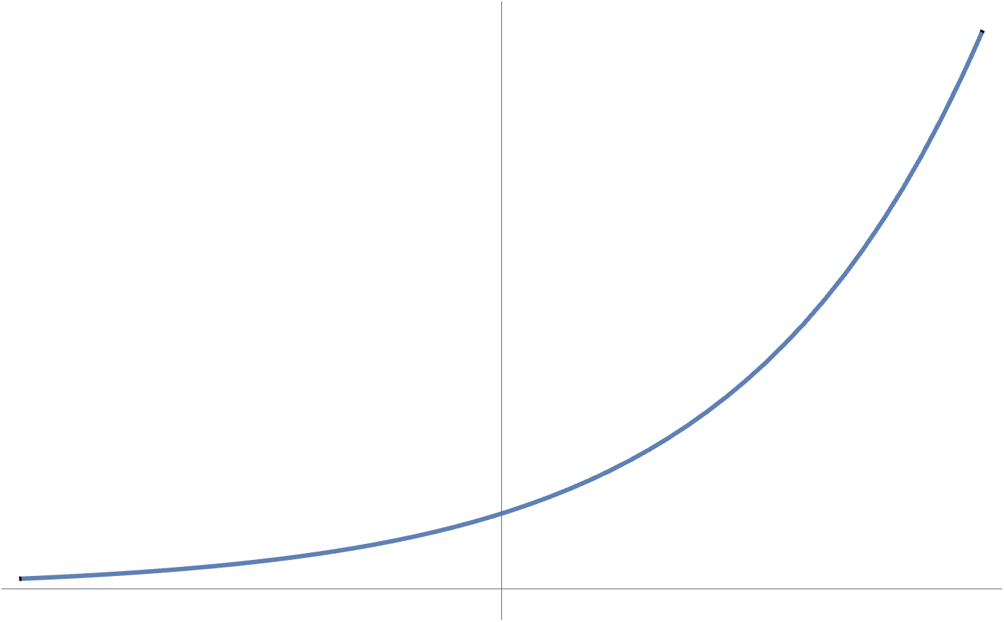
- It is possible that a convex function does not have a global optimum. Examples are \( F(x) = e^x \)
(fig. 1)
, which has an \( \inf \), but no lowest point.
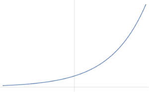
fig. 1. Exponential has no global optimum.
- Our discussion has been for unconstrained functions. For constrained problems (next topic) is not not necessarily true that \( \spacegrad F(\Bx) = 0 \) implies that \( \Bx \) is a global optimum, even for \( F \) convex.
As an example of a constrained problem consider
\begin{equation}\label{eqn:convexOptimizationLecture8:n}
\begin{aligned}
\min &2 x^2 + y^2 \\
x &\ge 3 \\
y &\ge 5.
\end{aligned}
\end{equation}
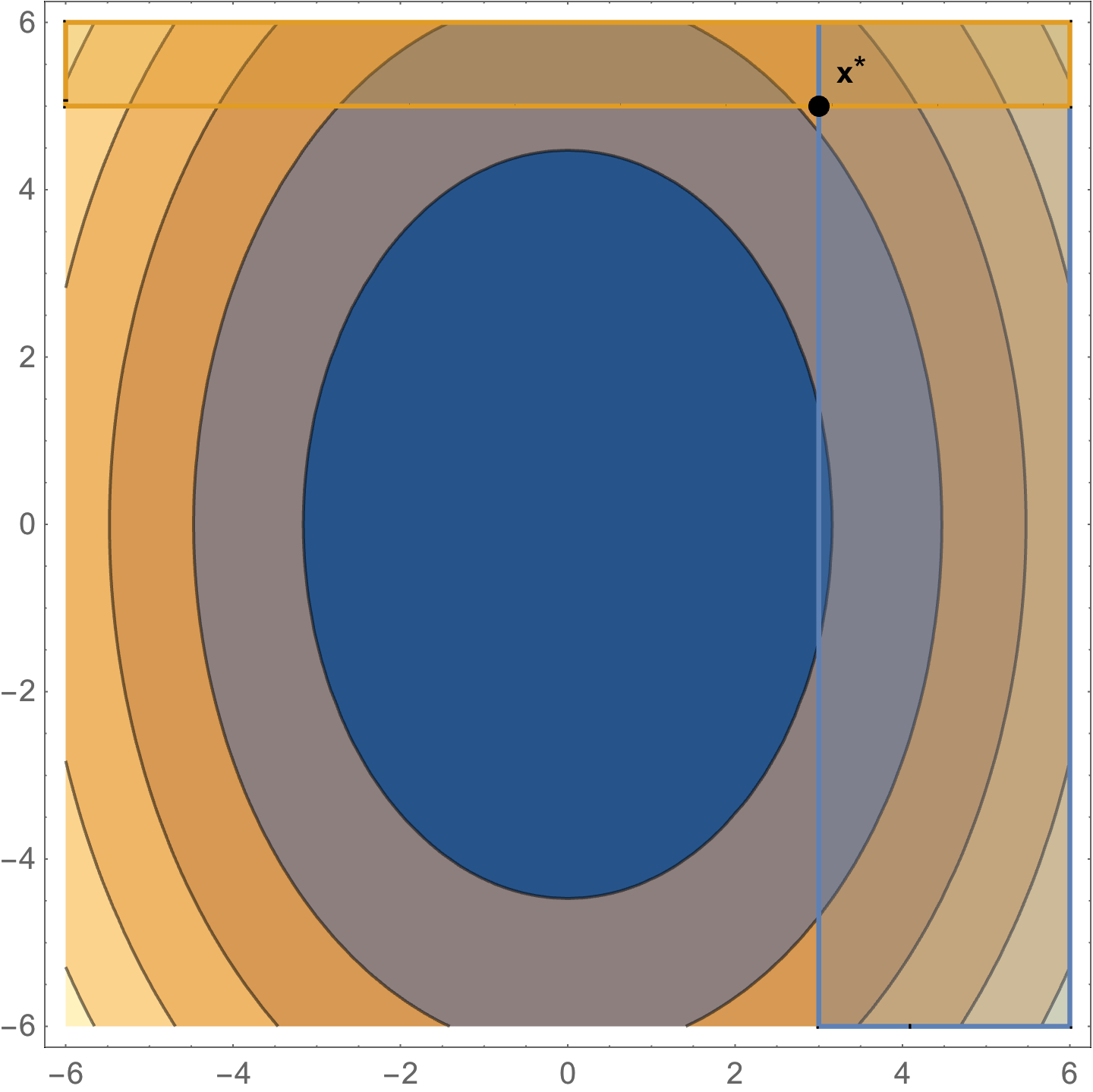
The level sets of this objective function are plotted in fig. 2. The optimal point is at \( \Bx^\conj = (3,5) \), where \( \spacegrad F \ne 0 \).
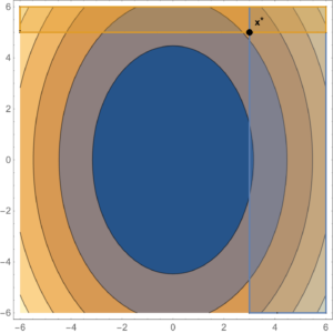
fig. 2. Constrained problem with optimum not at the zero gradient point.
Projection
Given \( \Bx \in \mathbb{R}^n, \By \in \mathbb{R}^p \), if \( h(\Bx,\By) \) is convex in \( \Bx, \By \), then
\begin{equation}\label{eqn:convexOptimizationLecture8:60}
F(\Bx_0) = \inf_\By h(\Bx_0,\By)
\end{equation}
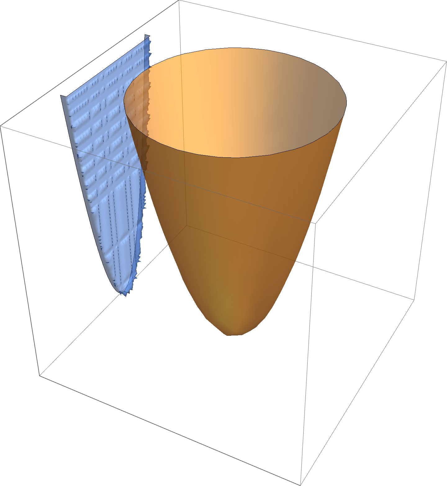
is convex in \( \Bx\), as sketched in fig. 3.
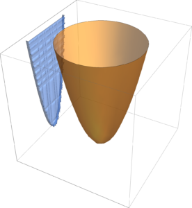
fig. 3. Epigraph of \( h \) is a filled bowl.
The intuition here is that shining light on the (filled) “bowl”. That is, the image of \( \textrm{epi} h \) on the \( \By = 0 \) screen which we will show is a convex set.
Proof:
Since \( h \) is convex in \( \begin{bmatrix} \Bx \\ \By \end{bmatrix} \in \textrm{dom} h \), then
\begin{equation}\label{eqn:convexOptimizationLecture8:80}
\textrm{epi} h = \setlr{ (\Bx,\By,t) | t \ge h(\Bx,\By), \begin{bmatrix} \Bx \\ \By \end{bmatrix} \in \textrm{dom} h },
\end{equation}
is a convex set.
We also have to show that the domain of \( F \) is a convex set. To show this note that
\begin{equation}\label{eqn:convexOptimizationLecture8:100}
\begin{aligned}
\textrm{dom} F
&= \setlr{ \Bx | \exists \By s.t. \begin{bmatrix} \Bx \\ \By \end{bmatrix} \in \textrm{dom} h } \\
&= \setlr{
\begin{bmatrix}
I_{n\times n} & 0_{n \times p}
\end{bmatrix}
\begin{bmatrix}
\Bx \\
\By
\end{bmatrix}
| \begin{bmatrix} \Bx \\ \By \end{bmatrix} \in \textrm{dom} h
}.
\end{aligned}
\end{equation}
This is an affine map of a convex set. Therefore \( \textrm{dom} F \) is a convex set.
\begin{equation}\label{eqn:convexOptimizationLecture8:120}
\begin{aligned}
\textrm{epi} F
&=
\setlr{ \begin{bmatrix} \Bx \\ \By \end{bmatrix} | t \ge \inf h(\Bx,\By), \Bx \in \textrm{dom} F, \By: \begin{bmatrix} \Bx \\ \By \end{bmatrix} \in \textrm{dom} h } \\
&=
\setlr{
\begin{bmatrix}
I & 0 & 0 \\
0 & 0 & 1
\end{bmatrix}
\begin{bmatrix}
\Bx \\
\By \\
t
\end{bmatrix}
|
t \ge h(\Bx,\By), \begin{bmatrix} \Bx \\ \By \end{bmatrix} \in \textrm{dom} h
}.
\end{aligned}
\end{equation}
Example:
The function
\begin{equation}\label{eqn:convexOptimizationLecture8:140}
F(\Bx) = \inf_{\By \in C} \Norm{ \Bx – \By },
\end{equation}
over \( \Bx \in \mathbb{R}^n, \By \in C \), ,is convex if \( C \) is a convex set. Reason:
- \( \Bx – \By \) is linear in \((\Bx, \By)\).
- \( \Norm{ \Bx – \By } \) is a convex function if the domain is a convex set
- The domain is \( \mathbb{R}^n \times C \). This will be a convex set if \( C \) is.
- \( h(\Bx, \By) = \Norm{\Bx -\By} \) is a convex function if \( \textrm{dom} h \) is a convex set. By setting \( \textrm{dom} h = \mathbb{R}^n \times C \), if \( C \) is convex, \( \textrm{dom} h \) is a convex set.
- \( F() \)
Composition of functions
Consider
\begin{equation}\label{eqn:convexOptimizationLecture8:160}
\begin{aligned}
F(\Bx) &= h(g(\Bx)) \\
\textrm{dom} F &= \setlr{ \Bx \in \textrm{dom} g | g(\Bx) \in \textrm{dom} h } \\
F &: \mathbb{R}^n \rightarrow \mathbb{R} \\
g &: \mathbb{R}^n \rightarrow \mathbb{R} \\
h &: \mathbb{R} \rightarrow \mathbb{R}.
\end{aligned}
\end{equation}
Cases:
- \( g \) is convex, \( h \) is convex and non-decreasing.
- \( g \) is convex, \( h \) is convex and non-increasing.
Show for 1D case ( \( n = 1 \)). Get to \( n > 1 \) by applying to all lines.
-
\begin{equation}\label{eqn:convexOptimizationLecture8:180}
\begin{aligned}
F'(x) &= h'(g(x)) g'(x) \\
F”(x) &=
h”(g(x)) g'(x) g'(x)
+
h'(g(x)) g”(x) \\
&=
h”(g(x)) (g'(x))^2
+
h'(g(x)) g”(x) \\
&=
\lr{ \ge 0 } \cdot \lr{ \ge 0 }^2 + \lr{ \ge 0 } \cdot \lr{ \ge 0 },
\end{aligned}
\end{equation}
since \( h \) is respectively convex, and non-decreasing.
-
\begin{equation}\label{eqn:convexOptimizationLecture8:180b}
\begin{aligned}
F'(x) =
\lr{ \ge 0 } \cdot \lr{ \ge 0 }^2 + \lr{ \le 0 } \cdot \lr{ \le 0 },
\end{aligned}
\end{equation}
since \( h \) is respectively convex, and non-increasing, and g is concave.
Extending to multiple dimensions
\begin{equation}\label{eqn:convexOptimizationLecture8:200}
\begin{aligned}
F(\Bx)
&= h(g(\Bx)) = h( g_1(\Bx), g_2(\Bx), \cdots g_k(\Bx) ) \\
g &: \mathbb{R}^n \rightarrow \mathbb{R} \\
h &: \mathbb{R}^k \rightarrow \mathbb{R}.
\end{aligned}
\end{equation}
is convex if \( g_i \) is convex for each \( i \in [1,k] \) and \( h \) is convex and non-decreasing in each argument.
Proof:
again assume \( n = 1 \), without loss of generality,
\begin{equation}\label{eqn:convexOptimizationLecture8:220}
\begin{aligned}
g &: \mathbb{R} \rightarrow \mathbb{R}^k \\
h &: \mathbb{R}^k \rightarrow \mathbb{R} \\
\end{aligned}
\end{equation}
\begin{equation}\label{eqn:convexOptimizationLecture8:240}
F”(\Bx)
=
\begin{bmatrix}
g_1(\Bx) & g_2(\Bx) & \cdots & g_k(\Bx)
\end{bmatrix}
\spacegrad^2 h(g(\Bx))
\begin{bmatrix}
g_1′(\Bx) \\ g_2′(\Bx) \\ \vdots \\ g_k'(\Bx)
\end{bmatrix}
+
\lr{ \spacegrad h(g(x)) }^\T
\begin{bmatrix}
g_1”(\Bx) \\ g_2”(\Bx) \\ \vdots \\ g_k”(\Bx)
\end{bmatrix}
\end{equation}
The Hessian is PSD.
Example:
\begin{equation}\label{eqn:convexOptimizationLecture8:260}
F(x) = \exp( g(x) ) = h( g(x) ),
\end{equation}
where \( g \) is convex is convex, and \( h(y) = e^y \). This implies that \( F \) is a convex function.
Example:
\begin{equation}\label{eqn:convexOptimizationLecture8:280}
F(x) = \inv{g(x)},
\end{equation}
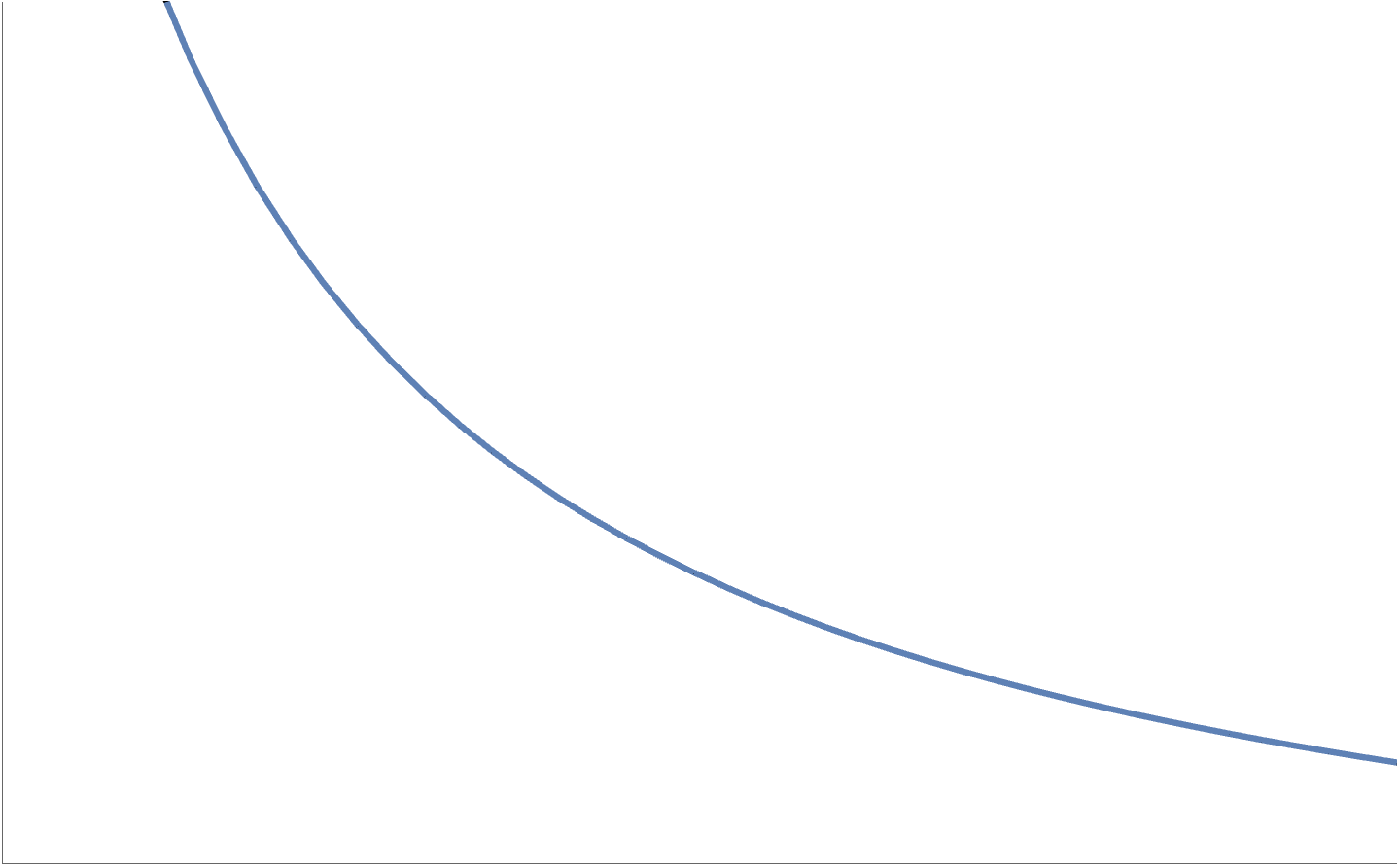
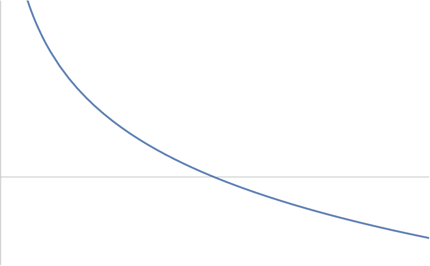
is convex if \( g(x) \) is concave and positive. The most simple such example of such a function is \( h(x) = 1/x, \textrm{dom} h = \mathbb{R}_{++} \), which is plotted in fig. 4.
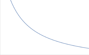
fig. 4. Inverse function is convex over positive domain.
Example:
\begin{equation}\label{eqn:convexOptimizationLecture8:300}
F(x) = – \sum_{i = 1}^n \log( -F_i(x) )
\end{equation}
is convex on \( \setlr{ x | F_i(x) < 0 \forall i } \) if all \( F_i \) are convex.
- Due to \( \textrm{dom} F \), \( -F_i(x) > 0 \,\forall x \in \textrm{dom} F \)
- \( \log(x) \) concave on \( \mathbb{R}_{++} \) so \( -\log \) convex also non-increasing (fig. 5).
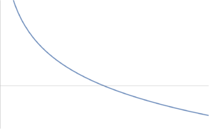
fig. 5. Negative logarithm convex over positive domain.
\begin{equation}\label{eqn:convexOptimizationLecture8:320}
F(x) = \sum h_i(x)
\end{equation}
but
\begin{equation}\label{eqn:convexOptimizationLecture8:340}
h_i(x) = -\log(-F_i(x)),
\end{equation}
which is a convex and non-increasing function (\(-\log\)), of a convex function \( -F_i(x) \). Each
\( h_i \) is convex, so this is a sum of convex functions, and is therefore convex.
Example:
Over \( \textrm{dom} F = S^n_{++} \)
\begin{equation}\label{eqn:convexOptimizationLecture8:360}
F(X) = \log \det X^{-1}
\end{equation}
To show that this is convex, check all lines in domain. A line in \( S^n_{++} \) is a 1D family of matrices
\begin{equation}\label{eqn:convexOptimizationLecture8:380}
\tilde{F}(t) = \log \det( \lr{X_0 + t H}^{-1} ),
\end{equation}
where \( X_0 \in S^n_{++}, t \in \mathbb{R}, H \in S^n \).
F9
For \( t \) small enough,
\begin{equation}\label{eqn:convexOptimizationLecture8:400}
X_0 + t H \in S^n_{++}
\end{equation}
\begin{equation}\label{eqn:convexOptimizationLecture8:420}
\begin{aligned}
\tilde{F}(t)
&= \log \det( \lr{X_0 + t H}^{-1} ) \\
&= \log \det\lr{ X_0^{-1/2} \lr{I + t X_0^{-1/2} H X_0^{-1/2} }^{-1} X_0^{-1/2} } \\
&= \log \det\lr{ X_0^{-1} \lr{I + t X_0^{-1/2} H X_0^{-1/2} }^{-1} } \\
&= \log \det X_0^{-1} + \log\det \lr{I + t X_0^{-1/2} H X_0^{-1/2} }^{-1} \\
&= \log \det X_0^{-1} – \log\det \lr{I + t X_0^{-1/2} H X_0^{-1/2} } \\
&= \log \det X_0^{-1} – \log\det \lr{I + t M }.
\end{aligned}
\end{equation}
If \( \lambda_i \) are eigenvalues of \( M \), then \( 1 + t \lambda_i \) are eigenvalues of \( I + t M \). i.e.:
\begin{equation}\label{eqn:convexOptimizationLecture8:440}
\begin{aligned}
(I + t M) \Bv
&=
I \Bv + t \lambda_i \Bv \\
&=
(1 + t \lambda_i) \Bv.
\end{aligned}
\end{equation}
This gives
\begin{equation}\label{eqn:convexOptimizationLecture8:460}
\begin{aligned}
\tilde{F}(t)
&= \log \det X_0^{-1} – \log \prod_{i = 1}^n (1 + t \lambda_i) \\
&= \log \det X_0^{-1} – \sum_{i = 1}^n \log (1 + t \lambda_i)
\end{aligned}
\end{equation}
- \( 1 + t \lambda_i \) is linear in \( t \).
- \( -\log \) is convex in its argument.
- sum of convex function is convex.
Example:
\begin{equation}\label{eqn:convexOptimizationLecture8:480}
F(X) = \lambda_\max(X),
\end{equation}
is convex on \( \textrm{dom} F \in S^n \)
(a)
\begin{equation}\label{eqn:convexOptimizationLecture8:500}
\lambda_{\max} (X) = \sup_{\Norm{\Bv}_2 \le 1} \Bv^\T X \Bv,
\end{equation}
\begin{equation}\label{eqn:convexOptimizationLecture8:520}
\begin{bmatrix}
\lambda_1 & & & \\
& \lambda_2 & & \\
& & \ddots & \\
& & & \lambda_n
\end{bmatrix}
\end{equation}
Recall that a decomposition
\begin{equation}\label{eqn:convexOptimizationLecture8:540}
\begin{aligned}
X &= Q \Lambda Q^\T \\
Q^\T Q = Q Q^\T = I
\end{aligned}
\end{equation}
can be used for any \( X \in S^n \).
(b)
Note that \( \Bv^\T X \Bv \) is linear in \( X \). This is a max of a number of linear (and convex) functions, so it is convex.
Last example:
(non-symmetric matrices)
\begin{equation}\label{eqn:convexOptimizationLecture8:560}
F(X) = \sigma_\max(X),
\end{equation}
is convex on \( \textrm{dom} F = \mathbb{R}^{m \times n} \). Here
\begin{equation}\label{eqn:convexOptimizationLecture8:580}
\sigma_\max(X) = \sup_{\Norm{\Bv}_2 = 1} \Norm{X \Bv}_2
\end{equation}
This is called an operator norm of \( X \). Using the SVD
\begin{equation}\label{eqn:convexOptimizationLecture8:600}
\begin{aligned}
X &= U sectionigma V^\T \\
U &= \mathbb{R}^{m \times r} \\
sectionigma &\in \mathrm{diag} \in \mathbb{R}{ r \times r } \\
V^T &\in \mathbb{R}^{r \times n}.
\end{aligned}
\end{equation}
Have
\begin{equation}\label{eqn:convexOptimizationLecture8:620}
\Norm{X \Bv}_2^2
=
\Norm{ U sectionigma V^\T \Bv }_2^2
=
\Bv^\T V sectionigma U^\T U sectionigma V^\T \Bv
=
\Bv^\T V sectionigma sectionigma V^\T \Bv
=
\Bv^\T V sectionigma^2 V^\T \Bv
=
\tilde{\Bv}^\T sectionigma^2 \tilde{\Bv},
\end{equation}
where \( \tilde{\Bv} = \Bv^\T V \), so
\begin{equation}\label{eqn:convexOptimizationLecture8:640}
\Norm{X \Bv}_2^2
=
\sum_{i = 1}^r \sigma_i^2 \Norm{\tilde{\Bv}}
\le \sigma_\max^2 \Norm{\tilde{\Bv}}^2,
\end{equation}
or
\begin{equation}\label{eqn:convexOptimizationLecture8:660}
\Norm{X \Bv}_2
\le \sqrt{ \sigma_\max^2 } \Norm{\tilde{\Bv}}
\le
\sigma_\max.
\end{equation}
Set \( \Bv \) to the right singular value of \( X \) to get equality.
References
[1] Stephen Boyd and Lieven Vandenberghe. Convex optimization. Cambridge university press, 2004.
Like this:
Like Loading...


 Having to condense all my latex onto a single line is one of the reasons I switched from the default wordpress latex engine to mathjax. It was annoying enough that I started paying for my wordpress hosting, and stopped posting on my old free peeterjoot.wordpress.com blog. Using KaTex and having to go back to single line latex would suck!