[Click here for a PDF of this post with nicer formatting]
Previously, the time domain MNA equations and first steps at producing the Harmonic Balance equations were performed. That was a frequency domain analysis with an assumed Fourier solution associated with discrete time sampling.
The next goal is to put this in block matrix form. First introducing discrete time sampling vectors
\begin{equation}\label{eqn:diodeRLCSample:100}
\Bv_a =
\begin{bmatrix}
v_a(t_{-N}) \\
v_a(t_{1-N}) \\
\vdots \\
v_a(t_{N-1}) \\
v_a(t_{N}) \\
\end{bmatrix}, \qquad
\Bu_a =
\begin{bmatrix}
u_b(t_{-N}) \\
u_b(t_{1-N}) \\
\vdots \\
u_b(t_{N-1}) \\
u_b(t_{N}) \\
\end{bmatrix}, \qquad
\Bw_a =
\begin{bmatrix}
w_c(t_{-N}) \\
w_c(t_{1-N}) \\
\vdots \\
w_c(t_{N-1}) \\
w_c(t_{N}) \\
\end{bmatrix},
\end{equation}
and Fourier component vectors
\begin{equation}\label{eqn:diodeRLCSample:120}
\BV_a =
\begin{bmatrix}
V^{(a)}_{-N} \\
V^{(a)}_{1-N} \\
\vdots \\
V^{(a)}_{N-1} \\
V^{(a)}_{N} \\
\end{bmatrix}, \qquad
\BU_b =
\begin{bmatrix}
U^{(b)}_{-N} \\
U^{(b)}_{1-N} \\
\vdots \\
U^{(b)}_{N-1} \\
U^{(b)}_{N} \\
\end{bmatrix}, \qquad
\BW_c =
\begin{bmatrix}
W^{(c)}_{-N} \\
W^{(c)}_{1-N} \\
\vdots \\
W^{(c)}_{N-1} \\
W^{(c)}_{N} \\
\end{bmatrix}.
\end{equation}
With \( \alpha = e^{ 2 \pi j /(2 N + 1) } \), and
\begin{equation}\label{eqn:diodeRLCSample:140}
\BF =
\begin{bmatrix}
\alpha^{ N N } & \alpha^{ \lr{N-1} N } & \cdots & 1 & \cdots & \alpha^{ -\lr{N-1} N } & \alpha^{ -N N } \\
\alpha^{ N \lr{N-1} } & \alpha^{ \lr{N-1} \lr{N-1} } & \cdots & 1 & \cdots & \alpha^{ -\lr{N-1} \lr{N-1} } & \alpha^{ -N \lr{N-1} } \\
\vdots & \vdots & \vdots & \vdots & \vdots & \vdots & \vdots \\
1 & 1 & 1 & 1 & 1 & 1 & 1 \\
\vdots & \vdots & \vdots & \vdots & \vdots & \vdots & \vdots \\
\alpha^{ -N \lr{N-1} } & \alpha^{ -\lr{N-1} \lr{N-1} } & \cdots & 1 & \cdots & \alpha^{ {N-1} \lr{N-1} } & \alpha^{ N \lr{N-1} } \\
\alpha^{ -N N } & \alpha^{ -N N } & \cdots & 1 & \cdots & \alpha^{ \lr{N-1} N } & \alpha^{ N N } \\
\end{bmatrix},
\end{equation}
in each case the time domain sampling vectors are related to the Fourier components by relations of the form
\begin{equation}\label{eqn:diodeRLCSample:160}
\Bx = \BF \BX.
\end{equation}
Block matrix form, with physical parameter ordering
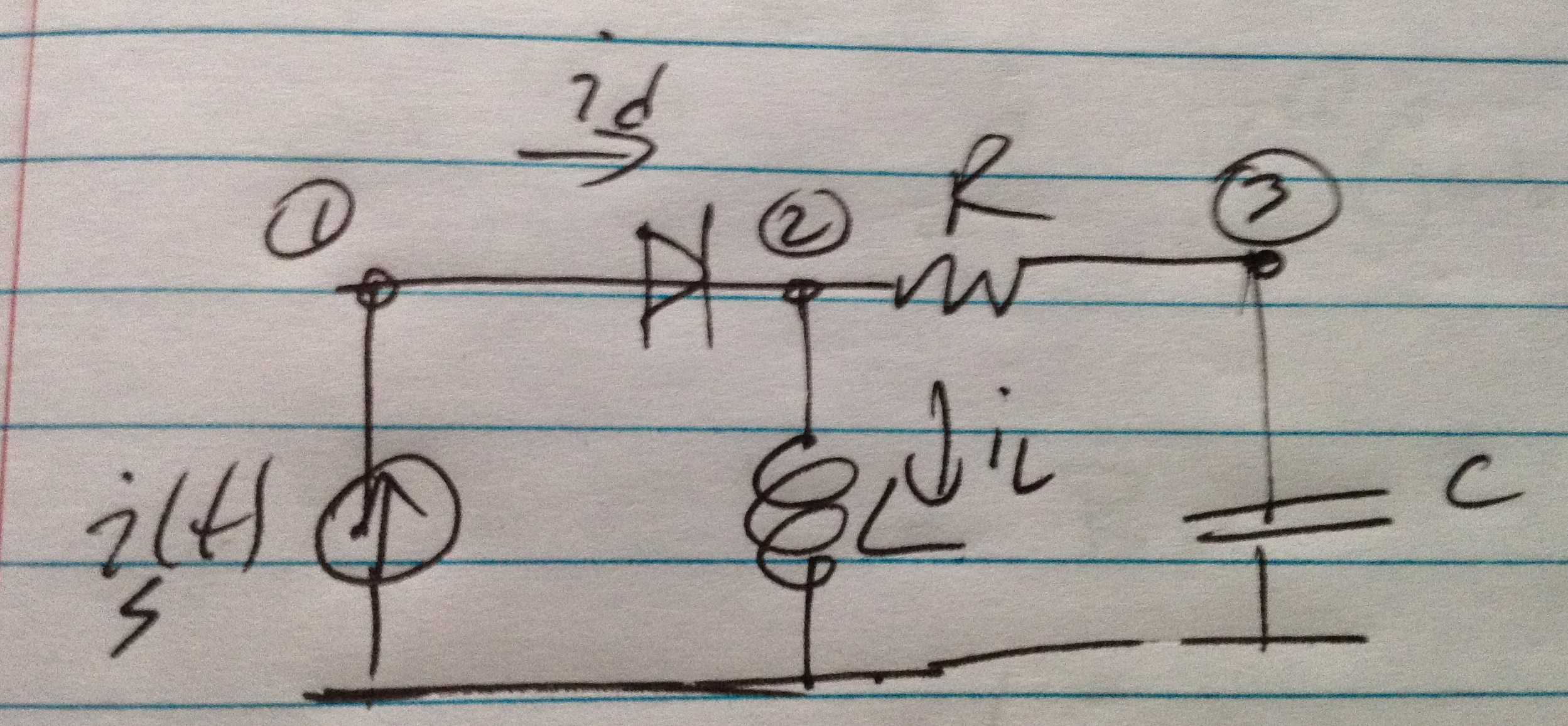
To understand how to put \ref{eqn:diodeRLCSample:240} in block matrix form, it is helpful to consider a specific example. Consider again the specific example of the RLC circuit above, which has the form
\begin{equation}\label{eqn:diodeRLCSample:260}
\begin{bmatrix}
0 & 0 & 0 & 0 \\
0 & Z & -Z & 1 \\
0 & -Z & Z + j \omega_0 n C & 0 \\
0 & -1 & 0 & + j \omega_0 n L \\
\end{bmatrix}
\begin{bmatrix}
V_n^{(1)} \\
V_n^{(2)} \\
V_n^{(3)} \\
I_n^{(L)} \\
\end{bmatrix}
=
\begin{bmatrix}
I_n^{(1)} \\
I_n^{(2)} \\
I_n^{(3)} \\
I_n^{(4)} \\
\end{bmatrix}
\end{equation}
Here the \( I^{(i)} \) terms are the DFT representations of both the linear and non-linear sources.
Suppose for example that \( N = 1 \). One way to write \ref{eqn:diodeRLCSample:260} would be
\begin{equation}\label{eqn:diodeRLCSample:320}
\begin{aligned}
&
\begin{bmatrix}
I_{-1}^{(1)} \\
I_0^{(1)} \\
I_{1}^{(1)} \\
I_{-1}^{(2)} \\
I_0^{(2)} \\
I_{1}^{(2)} \\
I_{-1}^{(3)} \\
I_0^{(3)} \\
I_{1}^{(3)} \\
I_{-1}^{(4)} \\
I_0^{(4)} \\
I_{1}^{(4)} \\
\end{bmatrix}
=
\left[
\begin{array}{c|c|c|c}
\begin{matrix}
0 & 0 & 0 \\
0 & 0 & 0 \\
0 & 0 & 0 \\
\end{matrix} &
\begin{matrix}
0 & 0 & 0 \\
0 & 0 & 0 \\
0 & 0 & 0 \\
\end{matrix} &
\begin{matrix}
0 & 0 & 0 \\
0 & 0 & 0 \\
0 & 0 & 0 \\
\end{matrix} &
\begin{matrix}
0 & 0 & 0 \\
0 & 0 & 0 \\
0 & 0 & 0 \\
\end{matrix} \\ \hline
\begin{matrix}
0 & 0 & 0 \\
0 & 0 & 0 \\
0 & 0 & 0 \\
\end{matrix} &
\begin{matrix}
Z & 0 & 0 \\
0 & Z & 0 \\
0 & 0 & Z \\
\end{matrix} &
\begin{matrix}
-Z & 0 & 0 \\
0 & -Z & 0 \\
0 & 0 & -Z \\
\end{matrix} &
\begin{matrix}
1 & 0 & 0 \\
0 & 1 & 0 \\
0 & 0 & 1 \\
\end{matrix} \\ \hline
\begin{matrix}
0 & 0 & 0 \\
0 & 0 & 0 \\
0 & 0 & 0 \\
\end{matrix} &
\begin{matrix}
-Z & 0 & 0 \\
0 & -Z & 0 \\
0 & 0 & -Z \\
\end{matrix} &
\begin{matrix}
Z & 0 & 0 \\
0 & Z & 0 \\
0 & 0 & Z \\
\end{matrix} &
\begin{matrix}
0 & 0 & 0 \\
0 & 0 & 0 \\
0 & 0 & 0 \\
\end{matrix} \\ \hline
\begin{matrix}
0 & 0 & 0 \\
0 & 0 & 0 \\
0 & 0 & 0 \\
\end{matrix} &
\begin{matrix}
-1 & 0 & 0 \\
0 & -1 & 0 \\
0 & 0 & -1 \\
\end{matrix} &
\begin{matrix}
0 & 0 & 0 \\
0 & 0 & 0 \\
0 & 0 & 0 \\
\end{matrix} &
\begin{matrix}
0 & 0 & 0 \\
0 & 0 & 0 \\
0 & 0 & 0 \\
\end{matrix} \\
\end{array}
\right]
\begin{bmatrix}
V_{-1}^{(1)} \\
V_{0}^{(1)} \\
V_{1}^{(1)} \\
V_{-1}^{(2)} \\
V_{0}^{(2)} \\
V_{1}^{(2)} \\
V_{-1}^{(3)} \\
V_{0}^{(3)} \\
V_{1}^{(3)} \\
I_{-1}^{(L)} \\
I_{0}^{(L)} \\
I_{1}^{(L)} \\
\end{bmatrix} \\
&+
\left[
\begin{array}{c|c|c|c}
\begin{matrix}
0 & 0 & 0 \\
0 & 0 & 0 \\
0 & 0 & 0 \\
\end{matrix} &
\begin{matrix}
0 & 0 & 0 \\
0 & 0 & 0 \\
0 & 0 & 0 \\
\end{matrix} &
\begin{matrix}
0 & 0 & 0 \\
0 & 0 & 0 \\
0 & 0 & 0 \\
\end{matrix} &
\begin{matrix}
0 & 0 & 0 \\
0 & 0 & 0 \\
0 & 0 & 0 \\
\end{matrix} \\ \hline
\begin{matrix}
0 & 0 & 0 \\
0 & 0 & 0 \\
0 & 0 & 0 \\
\end{matrix} &
\begin{matrix}
0 & 0 & 0 \\
0 & 0 & 0 \\
0 & 0 & 0 \\
\end{matrix} &
\begin{matrix}
0 & 0 & 0 \\
0 & 0 & 0 \\
0 & 0 & 0 \\
\end{matrix} &
\begin{matrix}
0 & 0 & 0 \\
0 & 0 & 0 \\
0 & 0 & 0 \\
\end{matrix} \\ \hline
\begin{matrix}
0 & 0 & 0 \\
0 & 0 & 0 \\
0 & 0 & 0 \\
\end{matrix} &
\begin{matrix}
0 & 0 & 0 \\
0 & 0 & 0 \\
0 & 0 & 0 \\
\end{matrix} &
\begin{matrix}
j \omega_0 (-1) C & 0 & 0 \\
0 & j \omega_0 (0) C & 0 \\
0 & 0 & j \omega_0 (1) C \\
\end{matrix} &
\begin{matrix}
0 & 0 & 0 \\
0 & 0 & 0 \\
0 & 0 & 0 \\
\end{matrix} \\ \hline
\begin{matrix}
0 & 0 & 0 \\
0 & 0 & 0 \\
0 & 0 & 0 \\
\end{matrix} &
\begin{matrix}
0 & 0 & 0 \\
0 & 0 & 0 \\
0 & 0 & 0 \\
\end{matrix} &
\begin{matrix}
0 & 0 & 0 \\
0 & 0 & 0 \\
0 & 0 & 0 \\
\end{matrix} &
\begin{matrix}
j \omega_0 (-1) L & 0 & 0 \\
0 & j \omega_0 (0) L & 0 \\
0 & 0 & j \omega_0 (1) L \\
\end{matrix} \\
\end{array}
\right]
\begin{bmatrix}
V_{-1}^{(1)} \\
V_{0}^{(1)} \\
V_{1}^{(1)} \\
V_{-1}^{(2)} \\
V_{0}^{(2)} \\
V_{1}^{(2)} \\
V_{-1}^{(3)} \\
V_{0}^{(3)} \\
V_{1}^{(3)} \\
I_{-1}^{(L)} \\
I_{0}^{(L)} \\
I_{1}^{(L)} \\
\end{bmatrix} \\
\end{aligned}
\end{equation}
With a vector of fourier coeffient vectors
\begin{equation}\label{eqn:diodeRLCSample:280}
\BV =
\begin{bmatrix}
\BV^{(1)} \\
\BV^{(2)} \\
\BV^{(3)} \\
\BI^{(L)}
\end{bmatrix}, \qquad
\BI =
\begin{bmatrix}
\BI^{(1)} \\
\BI^{(2)} \\
\BI^{(3)} \\
\BI^{(4)}
\end{bmatrix}.
\end{equation}
and a \( (2 N + 1) \times (2 N + 1) \) matrix of indexes
\begin{equation}\label{eqn:diodeRLCSample:220}
\BN =
\begin{bmatrix}
-N & & & & \\
& 1-N & & & \\
& & \ddots & & \\
& & & N-1 & \\
& & & & N \\
\end{bmatrix},
\end{equation}
the complete block diagonalization is
\begin{equation}\label{eqn:diodeRLCSample:300}
\boxed{
{\begin{bmatrix}
g_{rs} \BI_{2 N + 1} +
j \omega_0 c_{rs} \BN
\end{bmatrix}
}_{rs}
\BV
=
\BI.
}
\end{equation}
Block matrix form, with frequency ordering
It turns out that a better way of ordering the vector of Fourier components is using a frequency ordering that interleaves the physical parameters. With such an ordering the DFT MNA equations are
\begin{equation}\label{eqn:diodeRLCSample:340}
\begin{aligned}
\BI =
&\begin{bmatrix}
I_{-1}^{(1)} \\
I_{-1}^{(2)} \\
I_{-1}^{(3)} \\
I_{-1}^{(4)} \\
I_0^{(1)} \\
I_0^{(2)} \\
I_0^{(3)} \\
I_0^{(4)} \\
I_{1}^{(1)} \\
I_{1}^{(2)} \\
I_{1}^{(3)} \\
I_{1}^{(4)} \\
\end{bmatrix}
+
\left[
\begin{array}{c|c|c}
\begin{matrix}
0 & 0 & 0 & 0 \\
0 & Z & -Z & 1 \\
0 & -Z & Z & 0 \\
0 & -1 & 0 & 0 \\
\end{matrix} & 0 & 0 \\ \hline
0 &
\begin{matrix}
0 & 0 & 0 & 0 \\
0 & Z & -Z & 1 \\
0 & -Z & Z & 0 \\
0 & -1 & 0 & 0 \\
\end{matrix} & 0 \\ \hline
0 & 0 &
\begin{matrix}
0 & 0 & 0 & 0 \\
0 & Z & -Z & 1 \\
0 & -Z & Z & 0 \\
0 & -1 & 0 & 0 \\
\end{matrix} \\
\end{array}
\right]
\begin{bmatrix}
V_{-1}^{(1)} \\
V_{-1}^{(2)} \\
V_{-1}^{(3)} \\
I_{-1}^{(L)} \\
V_{0}^{(1)} \\
V_{0}^{(2)} \\
V_{0}^{(3)} \\
I_{0}^{(L)} \\
V_{1}^{(1)} \\
V_{1}^{(2)} \\
V_{1}^{(3)} \\
I_{1}^{(L)} \\
\end{bmatrix} \\
&+
j \omega_0
\left[
\begin{array}{c|c|c}
(-1)
\begin{bmatrix}
0 & 0 & 0 & 0 \\
0 & 0 & 0 & 0 \\
0 & 0 & C & 0 \\
0 & 0 & 0 & L \\
\end{bmatrix} & 0 & 0 \\ \hline
0 &
(0)
\begin{bmatrix}
0 & 0 & 0 & 0 \\
0 & 0 & 0 & 0 \\
0 & 0 & C & 0 \\
0 & 0 & 0 & L \\
\end{bmatrix} & 0 \\ \hline
0 & 0 &
(1)
\begin{bmatrix}
0 & 0 & 0 & 0 \\
0 & 0 & 0 & 0 \\
0 & 0 & C & 0 \\
0 & 0 & 0 & L \\
\end{bmatrix} \\
\end{array}
\right]
\begin{bmatrix}
V_{-1}^{(1)} \\
V_{-1}^{(2)} \\
V_{-1}^{(3)} \\
I_{-1}^{(L)} \\
V_{0}^{(1)} \\
V_{0}^{(2)} \\
V_{0}^{(3)} \\
I_{0}^{(L)} \\
V_{1}^{(1)} \\
V_{1}^{(2)} \\
V_{1}^{(3)} \\
I_{1}^{(L)} \\
\end{bmatrix} \\
\end{aligned}
\end{equation}
This ordering matches that of [1].
Representing the linear sources
Assuming real sources with frequencies that are only multiples of the fundamental harmonic, a reasonable way to represent them in storage is with a pair of matrices
\begin{equation}\label{eqn:diodeRLCSample:360}
\begin{bmatrix}
\BI \sim \BB \Bomega
\end{bmatrix}.
\end{equation}
If \( R \) is the dimension of \(\BG\) and \( \BC \), then \( \BB \) is a \( R \times S \) dimension matrix, where \( S \) is the sum of
- 1, if there are any DC sources, plus
- 2 times the number of unique frequency sources.
For example, if there is a DC source and one AC source with frequency \( \nu \), then for column vectors \( \Bb_i \) this pair is of the form
\begin{equation}\label{eqn:diodeRLCSample:380}
\BU \Bomega =
\begin{bmatrix}
\Bb_{-1} & \Bb_0 & \Bb_1
\end{bmatrix}
\begin{bmatrix}
– 2 \pi \nu \\
0 \\
2 \pi \nu
\end{bmatrix}.
\end{equation}
This representation produces the time domain representation exactly when there are only DC sources, and can be used to construct the Fourier coefficients by inspection when there are AC sources. For example, for \( N = 1 \) in the example above, the Fourier coefficent vector is
\begin{equation}\label{eqn:diodeRLCSample:400}
\BI
=
\begin{bmatrix}
\Bb_{-1} \\
\Bb_{0} \\
\Bb_{1} \\
\end{bmatrix}.
\end{equation}
If \( N = 2 \) was used, then we would have instead
\begin{equation}\label{eqn:diodeRLCSample:420}
\BI
=
\begin{bmatrix}
\Bzero \\
\Bb_{-1} \\
\Bb_{0} \\
\Bb_{1} \\
\Bzero \\
\end{bmatrix}.
\end{equation}
Representing non-linear sources
The time domain MNA fig. 1.
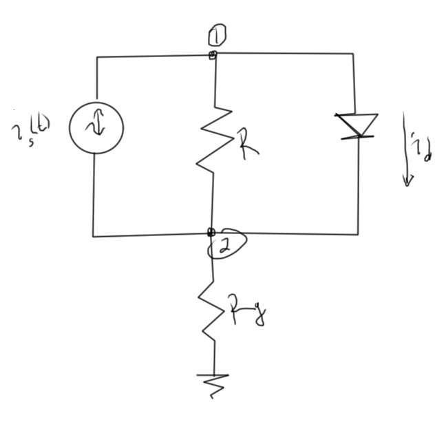
fig. 1. Simple diode circuit
With \( Z = 1/R, Z_g = 1/R_g \), the KCL equations are
- \( \lr{ v_1 – v_2 } Z_s = i_s – i_d \)
- \( \lr{ v_2 – v_1 } Z_s + v_2 Z_g = -i_s + i_d \)
Using the model \( i_d = I^{(0)} \lr{ e^{ (v_1 – v_2)/V_T } – 1 } \), with source \( i_s = I^{(s)} \cos( \omega_0 t ) \),
this has the block matrix form
\begin{equation}\label{eqn:diodeRLCSample:580}
\BG =
\begin{bmatrix}
Z_s & -Z_s \\
-Z_s & Z_s + Z_g \\
\end{bmatrix}, \qquad
\Bx =
\begin{bmatrix}
v_1(t) \\
v_2(t) \\
\end{bmatrix}
\end{equation}
\begin{equation}\label{eqn:diodeRLCSample:600}
\BB =
\begin{bmatrix}
I^{(s)}/2 & -I^{(0)} & I^{(s)}/2 \\
-I^{(s)}/2 & I^{(0)} & -I^{(s)}/2
\end{bmatrix}, \qquad
\Bu(t) =
\begin{bmatrix}
e^{-j \omega_0 t} \\
1 \\
e^{j \omega_0 t}
\end{bmatrix}
\end{equation}
\begin{equation}\label{eqn:diodeRLCSample:620}
\BD
=
\begin{bmatrix}
I^{(0)} \\
-I^{(0)}
\end{bmatrix}, \qquad
\Bw(t) = e^{(v_1(t) – v_2(t))/V_T}.
\end{equation}
If \( E_n \) is the nth DFT coefficient for \( e(t) = e^{(v_1(t) – v_2(t))/V_T} \), then the DFT equations for the \( N = 1 \) DFT is
\begin{equation}\label{eqn:diodeRLCSample:640}
\begin{aligned}
\lr{ V_{-1}^{(1)} – V_{-1}^{(2)} } Z_s &= I^{(s)}/2 – I^{(0)} E_{-1} \\
\lr{ V_{-1}^{(2)} – V_{-1}^{(1)} } Z_s + V_{-1}^{(2)} Z_g &= -I^{(s)}/2 + I^{(0)} E_{-1} \\
\lr{ V_{0}^{(1)} – V_{0}^{(2)} } Z_s &= I^{(0)} – I^{(0)} E_{0} \\
\lr{ V_{0}^{(2)} – V_{0}^{(1)} } Z_s + V_{0}^{(2)} Z_g &= -I^{(0)} + I^{(0)} E_{0} \\
\lr{ V_{1}^{(1)} – V_{1}^{(2)} } Z_s &= I^{(s)}/2 – I^{(0)} E_{1} \\
\lr{ V_{1}^{(2)} – V_{1}^{(1)} } Z_s + V_{1}^{(2)} Z_g &= -I^{(s)}/2 + I^{(0)} E_{1}
\end{aligned}
\end{equation}
Let \( \Bb = [ \Bb_{-1}\, \Bb_0\, \Bb_1 ] \), and \( \BD = [ \Bd_1 ] \). The block matrix equivalent form, by inspection, is
\begin{equation}\label{eqn:diodeRLCSample:660}
\begin{bmatrix}
\BG & 0 & 0 \\
0 & \BG & 0 \\
0 & 0 & \BG
\end{bmatrix}
\begin{bmatrix}
V_{-1}^{(1)} \\
V_{-1}^{(2)} \\
V_{0}^{(1)} \\
V_{0}^{(2)} \\
V_{1}^{(1)} \\
V_{1}^{(2)}
\end{bmatrix}
=
\begin{bmatrix}
\Bb_{-1} \\
\Bb_{0} \\
\Bb_{1} \\
\end{bmatrix}
+
\begin{bmatrix}
\Bd_1 E_{-1} \\
\Bd_1 E_{0} \\
\Bd_1 E_{1}
\end{bmatrix}.
\end{equation}
This shows the stamping pattern required to form the non-linear portion of the Harmonic balance equations. The general pattern can be written as
\begin{equation}\label{eqn:diodeRLCSample:820}
\boxed{
\mathcal{G} \BV = \BI + \mathcal{I}(\BV),
}
\end{equation}
Here \( \mathcal{G} \) is block diagonal, and in general has blocks of \( \BG + j \omega_0 n \BC \). The matrix \( \BI \) was generated from the Fourier coeffients of all the linear sources, and \( \mathcal{I}(\BV) \) encodes all the non-linear contributions to the system.
More general non-linear structure, for multiple diodes
For the diode exponentials, these non-linear term will be of the form
\begin{equation}\label{eqn:diodeRLCSample:680}
\BD \Bw(t)
=
\begin{bmatrix}
\Bd_1 & \Bd_2 & \cdots & \Bd_S
\end{bmatrix}
\begin{bmatrix}
w_1(t) \\
w_2(t) \\
\vdots \\
w_S(t) \\
\end{bmatrix},
\end{equation}
where \( w_i(t) = \exp( (v_{i,1}(t) – v_{i,2}(t))/V_{T,i} ) \). If the DFT coordinates of these functions are \( E_n^{(i)} \), then the frequency domain representation is
\begin{equation}\label{eqn:diodeRLCSample:700}
\mathcal{I}(\BV)
=
\sum_{i = 1}^S
\begin{bmatrix}
\Bd_i E_{-N}^{(i)} \\
\Bd_i E_{1-N}^{(i)} \\
\vdots \\
\Bd_i E_{N-1}^{(i)} \\
\Bd_i E_{N}^{(i)} \\
\end{bmatrix}.
\end{equation}
This is a \( R (2 N + 1) \times 1 \) matrix, as expected.
The computation of these DFT coordinates is a bit messy since they are time dependent, and thus dependent on the (unknown) values of \( V_n^{(1)} \). Consider the above circuit as an example where we have
\begin{equation}\label{eqn:diodeRLCSample:720}
w(t) = \exp\lr{ (v_1(t) – v_2(t))/V_T }.
\end{equation}
The DFT inverse is
\begin{equation}\label{eqn:diodeRLCSample:740}
E_n = \sum_{k=-N}^N \exp\lr{ (v_1(t_k) – v_2(t_k))/V_T } e^{-j \omega_0 n t_k }.
\end{equation}
With \( \BE = ( E_{-N}, E_{1-N}, \cdots, E_{N-1}, E_N ) \), this is
\begin{equation}\label{eqn:diodeRLCSample:760}
\BE =
\inv{2 N + 1} \overline{{\BF}}
\begin{bmatrix}
\exp\lr{ (v_{-N}^{(1)} – v_{-N}^{(2)})/v_T } \\
\exp\lr{ (v_{1-N}^{(1)} – v_{1-N}^{(2)})/v_T } \\
\vdots \\
\exp\lr{ (v_{N-1}^{(1)} – v_{N-1}^{(2)})/v_T } \\
\exp\lr{ (v_{N}^{(1)} – v_{N}^{(2)})/v_T } \\
\end{bmatrix}
=
\inv{2 N + 1} \overline{{\BF}}
\begin{bmatrix}
\exp\lr{ {[\BF (\BV^{(1)} – \BV^{(2)})/v_T]}_{-N} } \\
\exp\lr{ {[\BF (\BV^{(1)} – \BV^{(2)})/v_T]}_{1-N} } \\
\vdots \\
\exp\lr{ {[\BF (\BV^{(1)} – \BV^{(2)})/v_T]}_{N-1} } \\
\exp\lr{ {[\BF (\BV^{(1)} – \BV^{(2)})/v_T]}_{N} }
\end{bmatrix}.
\end{equation}
With the introduction a term by term exponentiation operator
\begin{equation}\label{eqn:diodeRLCSample:780}
\exp[ \Bx ] =
\begin{bmatrix}
\exp(x_1) \\
\exp(x_2) \\
\vdots \\
\end{bmatrix},
\end{equation}
this one Fourier coefficient vector is
\begin{equation}\label{eqn:diodeRLCSample:800}
\BE =
\inv{2 N + 1} \overline{{\BF}}
\exp[ \BF (\BV^{(1)} – \BV^{(2)})/v_T ].
\end{equation}
This is now completely expressed in terms of the unknown Fourier component vectors, each a subset of the aggreggated “voltage”, range selectable with the Matlab operation \( \BV^{(i)} = \BV(i:R:end) \).
Newton’s method
In order to solve the system, Newton’s method on the Fourier coeffients is required. Solutions to \( \mathcal{F}(\BV) = 0 \) are sought, where
\begin{equation}\label{eqn:diodeRLCSample:840}
\mathcal{F}(\BV) = \mathcal{G} \BV – \BI – \mathcal{I}(\BV).
\end{equation}
Here the sources current vector DFT coordinates have been split into the linear contributions \( \BI \) and nonlinear contributions \( \mathcal{I} \) defined by \ref{eqn:diodeRLCSample:700}.
Working with ones-indexed coordinates of \( \BV = [V_k]_k \), where \( k \in [1, R(2 N + 1) ] \), the Jacobian is
\begin{equation}\label{eqn:diodeRLCSample:860}
\BJ = \mathcal{G} – {[ \PDi{V_s}{\mathcal{I}_r} ]}_{rs}.
\end{equation}
To calculate these partials we need the partials of the coordinates of \( \BE \) of
\ref{eqn:diodeRLCSample:800}. The kth coordinate of \( \BV^{(1)}, \BV^{(2)} \) in terms of the coordinates of the \( R(2 N + 1) \) vector of unknowns \( \BV \) are
\begin{equation}\label{eqn:diodeRLCSample:880}
\begin{aligned}
[\BV^{(1)}]_k &= V_{1 + (k-1) R} \\
[\BV^{(2)}]_k &= V_{2 + (k-1) R}
\end{aligned}
\end{equation}
Using summation convention, with sums over any repeated indexes implied, those coordinates are
\begin{equation}\label{eqn:diodeRLCSample:900}
E_r =
\inv{2 N + 1} \overline{{F}}_{r a}
\exp\lr{ F_{ab}
(
V_{1 + (b-1) R} –
V_{2 + (b-1) R}
)/v_T }.
\end{equation}
The partials now follow immediately
\begin{equation}\label{eqn:diodeRLCSample:920}
\PD{V_s}{E_r} =
\inv{2 N + 1} \inv{v_T} \overline{{F}}_{r a} F_{ab}
\exp\lr{ F_{ab}
(
V_{1 + (b-1) R} –
V_{2 + (b-1) R}
)/v_T }
\lr{
\delta_{s,1 + (b-1) R} –
\delta_{s,2 + (b-1) R}
}.
\end{equation}
Generalization
To generalize this, suppose that the diode exponential was associated with voltages spanning nodes \( m, n\) so that
\begin{equation}\label{eqn:diodeRLCSample:980}
\BE =
\inv{2 N + 1} \overline{{\BF}}
\exp[ \BF (\BV^{(m)} – \BV^{(n)})/v_T ].
\end{equation}
In this case, the coordinates of the physical “voltages” are
\begin{equation}\label{eqn:diodeRLCSample:1020}
\begin{aligned}
[\BV^{(m)}]_k &= V_{m + (k-1) R} \\
[\BV^{(n)}]_k &= V_{n + (k-1) R}
\end{aligned},
\end{equation}
so
\begin{equation}\label{eqn:diodeRLCSample:1040}
E_r =
\inv{2 N + 1} \overline{{F}}_{r a}
\exp\lr{ F_{ab}
(
V_{m + (b-1) R} –
V_{n + (b-1) R}
)/v_T }.
\end{equation}
The Jacobian partials are
\begin{equation}\label{eqn:diodeRLCSample:1060}
\PD{V_s}{E_r} =
\inv{2 N + 1} \inv{v_T} \overline{{F}}_{r a} F_{ab}
\exp\lr{ F_{ab}
(
V_{m + (b-1) R} –
V_{n + (b-1) R}
)/v_T }
\lr{
\delta_{s,m + (b-1) R} –
\delta_{s,n + (b-1) R}
}.
\end{equation}
Note that this Jacobian
\begin{equation}\label{eqn:diodeRLCSample:1080}
\BJ_\BE =
{
\begin{bmatrix}
\PD{V_s}{E_r}
\end{bmatrix}}_{rs}
\end{equation}
is a \( (2 N + 1) \times R(2N + 1) \) matrix.
The full Jacobian of \( \mathcal{I}(\BV) \) is
\begin{equation}\label{eqn:diodeRLCSample:1120}
\BJ_{\mathcal{I}}(\BV)
=
\sum_{i = 1}^S
\begin{bmatrix}
\Bd_i \PD{\BV}{E_{-N}^{(i)}} \\
\Bd_i \PD{\BV}{E_{1-N}^{(i)}} \\
\vdots \\
\Bd_i \PD{\BV}{E_{N-1}^{(i)}} \\
\Bd_i \PD{\BV}{E_{N}^{(i)}} \\
\end{bmatrix}.
\end{equation}
Where \( \PDi{\BV}{E_{k}^{(i)}} \) is the kth row of \( \BJ_{\BE^{(i)}} \). The complete Jacobian is
\begin{equation}\label{eqn:diodeRLCSample:1100}
\BJ = \mathcal{G} – \BJ_{\mathcal{I}}(\BV).
\end{equation}
References
Giannini and Giorgio Leuzzi. Nonlinear Microwave Circuit Design. Wiley Online Library, 2004.