This blog post is a text version of the video below, available in a few forms:
- [PDF]
- Google’s CensorShipTube
- Odysee
- WordPress with Mathjax, below.
We found previously that
\begin{equation}\label{eqn:solarellipse:20}
\mathbf{\hat{r}}’ = \inv{r} \mathbf{\hat{r}} \lr{ \mathbf{\hat{r}} \wedge \Bx’ }.
\end{equation}
Somewhat remarkably, we can use this identity to demonstrate that orbits governed gravitational force are elliptical (or parabolic, or hyperbolic.) This ends up being possible because the angular momentum of the system is a conserved quantity, and this immediately introduces angular momentum into the mix in a fundamental way. In particular,
\begin{equation}\label{eqn:solarellipse:40}
\mathbf{\hat{r}}’ = \inv{m r^2} \mathbf{\hat{r}} L,
\end{equation}
where we define the angular momentum bivector as
\begin{equation}\label{eqn:solarellipse:60}
L = \Bx \wedge \Bp.
\end{equation}
Our gravitational law is
\begin{equation}\label{eqn:solarellipse:80}
m \ddt{\Bv} = – G m M \frac{\mathbf{\hat{r}}}{r^2},
\end{equation}
or
\begin{equation}\label{eqn:solarellipse:100}
-\inv{G M} \ddt{\Bv} = \frac{\mathbf{\hat{r}}}{r^2}.
\end{equation}
Combining the gravitational law with our \( \mathbf{\hat{r}} \) derivative identity, we have
\begin{equation}\label{eqn:solarellipse:120}
\begin{aligned}
\ddt{ \mathbf{\hat{r}} }
&= \inv{m} \frac{\mathbf{\hat{r}}}{r^2} L \\
&= -\inv{G m M} \ddt{\Bv} L \\
&= -\inv{G m M} \lr{ \ddt{(\Bv L)} – \ddt{L} }.
\end{aligned}
\end{equation}
Since angular momentum is a constant of motion of the system, means that
\begin{equation}\label{eqn:solarellipse:140}
\ddt{L} = 0,
\end{equation}
our equation of motion is integratable
\begin{equation}\label{eqn:solarellipse:160}
\ddt{ \mathbf{\hat{r}} } = -\inv{G m M} \ddt{(\Bv L)}.
\end{equation}
Introducing a vector valued integration constant \( -\Be \), we have
\begin{equation}\label{eqn:solarellipse:180}
\mathbf{\hat{r}} = -\inv{G m M} \Bv L – \Be.
\end{equation}
We’ve transformed our second order differential equation to a first order equation, one that does not look easy to integrate one more time. Luckily, we do not have to integrate, and can partially solve this algebraically, enough to describe the orbit in a compact fashion.
Before trying that, it’s worth quickly demonstrating that this equation is not a multivector equation, but a vector equation, since the multivector \( \Bv L \) is, in fact, vector valued.
\begin{equation}\label{eqn:solarellipse:200}
\begin{aligned}
\Bv L
&= \Bv \lr{ \Bx \wedge (m \Bv) } \\
&\propto \mathbf{\hat{v}} \lr{ \mathbf{\hat{r}} \wedge \mathbf{\hat{v}} } \\
&= \mathbf{\hat{v}} \cdot \lr{ \mathbf{\hat{r}} \wedge \mathbf{\hat{v}} } + \mathbf{\hat{v}} \wedge \lr{ \mathbf{\hat{r}} \wedge \mathbf{\hat{v}} } \\
&= \mathbf{\hat{v}} \cdot \lr{ \mathbf{\hat{r}} \wedge \mathbf{\hat{v}} } \\
&= \lr{ \mathbf{\hat{v}} \cdot \mathbf{\hat{r}} } \mathbf{\hat{v}} – \mathbf{\hat{r}},
\end{aligned}
\end{equation}
which is a vector (i.e.: a vector that is directed along the portion of \( \Bx \) that is perpendicular to \( \Bv \).)
We can reduce \ref{eqn:solarellipse:180} to a scalar equation by dotting with \( \Bx = r \mathbf{\hat{r}} \), leaving
\begin{equation}\label{eqn:solarellipse:220}
\begin{aligned}
r
&= -\inv{G m M} \gpgradezero{ \Bx \Bv L } – \Bx \cdot \Be \\
&= -\inv{G m^2 M} \gpgradezero{ \Bx \Bp L } – \Bx \cdot \Be \\
&= -\inv{G m^2 M} \gpgradezero{ \lr{ \Bx \cdot \Bp + L } L } – \Bx \cdot \Be \\
&= -\inv{G m^2 M} L^2 – \Bx \cdot \Be,
\end{aligned}
\end{equation}
or
\begin{equation}\label{eqn:solarellipse:240}
r = -\frac{L^2}{G M m^2} – r e \cos\theta,
\end{equation}
or
\begin{equation}\label{eqn:solarellipse:260}
r \lr{ 1 + e \cos\theta } = -\frac{L^2}{G M m^2}.
\end{equation}
Observe that the RHS constant is a positive constant, since \( L^2 \le 0 \). This has the structure of a conic section, if we write
\begin{equation}\label{eqn:solarellipse:280}
-\frac{L^2}{G M m^2} = e d.
\end{equation}
This is an ellipse, for \( e \in [0,1) \), a parabola for \( e = 1 \), and hyperbola for \( e > 1 \) ([1] theorem 10.3.1).
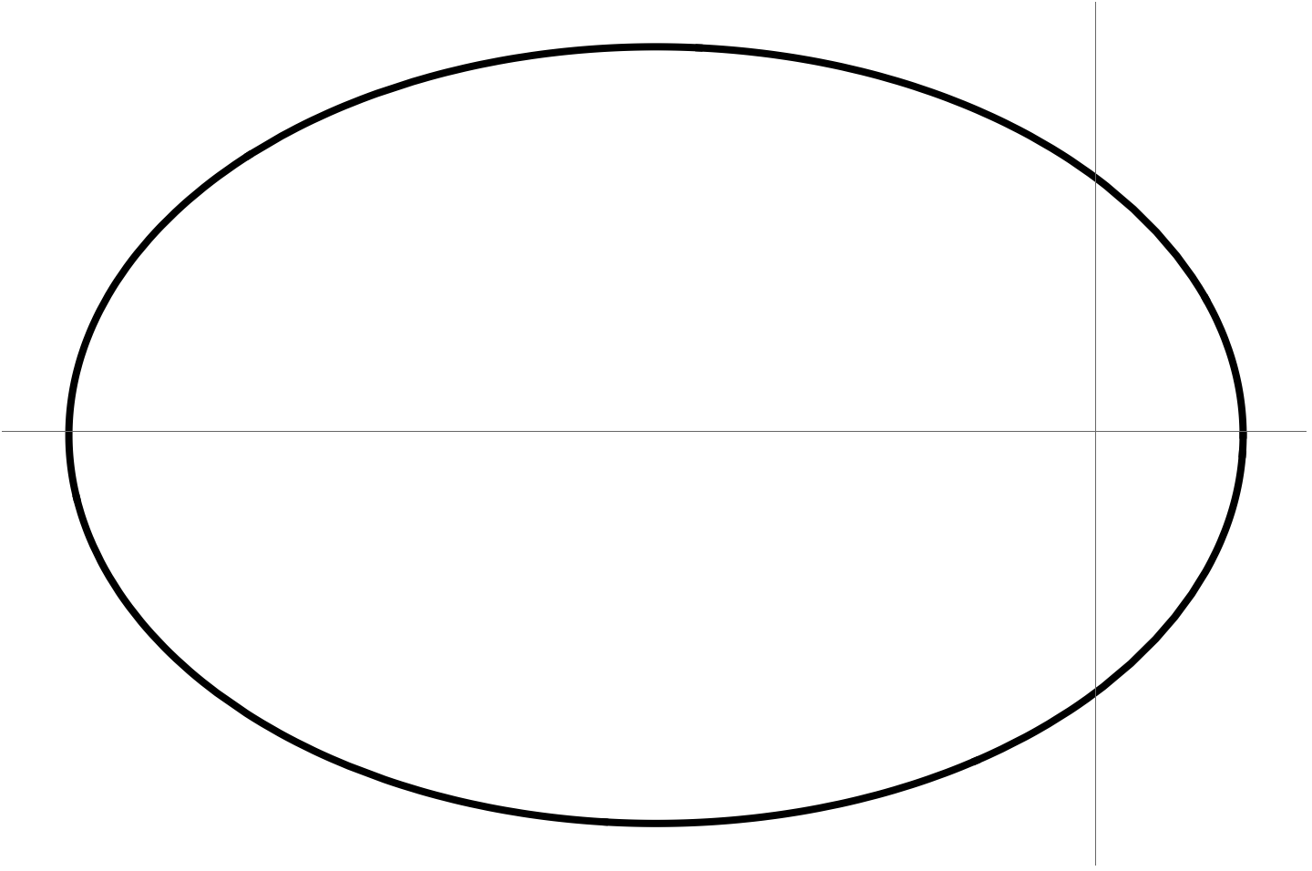
fig. 1. Ellipse with e = 0.75
In fig. 1 is a plot with \( e = 0.75 \) (changing \( d \) doesn’t change the shape of the figure, just the size.)
References
[1] S.L. Salas and E. Hille. Calculus: one and several variables. Wiley New York, 1990.