Remembrance day, a celebration and glorification of war

November 11, 2014 Incoherent ramblings

Today I received the following Remembrance day message at work:

“Every year on November 11th, Canadians pause for a moment of silence in remembrance of the men and women who have served our country during times of war, conflict and peace. More than 1,500,000 Canadians have served our country in this way and over 100,000 have paid the ultimate sacrifice.

They gave their lives and their futures for the freedoms we enjoy today.

At 11:00 a.m. today, please join me in observing one full minute of silence.

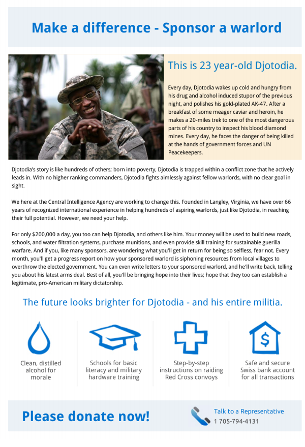
This illustrates precisely the sort of propaganda that is buried in this yearly celebration of war. Many people will object to my labeling of Remembrance day as a celebration of war, but I think that is an apt label.

We should remember the collective insanity that drove so many to send themselves off to be killed or kill. We should remember those who profited from the wars, and those who funded both sided. Let’s remember the Carnegies who concluded that there’s no better industry than war for profits and pleaded to Wilson to not end world war I too quickly. We should remember the massive propaganda campaigns to attempt to coerce people into fighting these wars. We should remember the disgusting lies that have been used again and again to justify wars that are later proven false. We should remember the US companies like Ford and IBM (my current employer!) that provided financial and resource backing to Hitler, without which his final atrocities would not have been possible. We should remember how every war has been an excuse for raising taxes to new peaks, raising nationalistic debt servitude at every turn (*). We should remember that civilians are the people most hurt by wars, and not focus our attentions on those soldiers that held the guns or were shot by them.

There are many things to remember, and if we are deluded into focusing our attention on the “sacrifices of soldiers”, who are pawns in the grand scheme of things, then we loose.

It is interesting to see just how transparent the Remembrance day propaganda can be. It is not just the glorification of the soldiers who were killed and did their killing. We are asked specifically to also glorify the people that “serve” Canada in it’s day to day waging of what amounts to US imperialistic warfare in times of peace.

Ron Paul’s recent commentary on Canada’s current war mongering nature was very apt.  We should remember that the aggressions that happen in our names have consequences.

If it were not for acceptance of the sorts of patriotic drivel that we see on Remembrance day, and patriotism conditioning events like the daily standing for the national anthem, perhaps a few less people would be so willing to fight wars for or against governments that are not worth obeying.

We give governments power by sheepish compliance. This service is to an entity that is a figment of our collective agreement.

Today I’ll actually just remember my dad. He is the only person I knew that saw through the social conditioning of Remembrance day and so aptly identified it as a propaganda event.


Footnotes:

(*) I’m not sure how definitive the debtclock link above is, nor it’s sources.  Here’s a newer Canadian debt-clock.  That site is currently also vague about it’s sources, citing “Canadian Government Data” without specifying them, nor linking to them.

ECE1254H Modeling of Multiphysics Systems. Lecture 14: Backward Euler method and trapezoidal methods. Taught by Prof. Piero Triverio

November 10, 2014 ece1254 , , ,

[Click here for a PDF of this post with nicer formatting]

Disclaimer

Peeter’s lecture notes from class. These may be incoherent and rough.

Backward Euler method

Discretized time dependent partial differential equations were seen to have the form

\begin{equation}\label{eqn:multiphysicsL14:20}
G \Bx(t) + C \dot{\Bx}(t) = B \Bu(t),
\end{equation}

where \( G, C, B \) are matrices, and \( \Bu(t) \) is a vector of sources.

The backward Euler method augments \ref{eqn:multiphysicsL14:20} with an initial condition. For a one dimensional system such an initial condition could a zero time specification

\begin{equation}\label{eqn:multiphysicsL14:40}
G x(t) + C \dot{x}(t) = B u(t),
\end{equation}
\begin{equation}\label{eqn:multiphysicsL14:60}
x(0) = x_0
\end{equation}

Discretizing time as in fig. 1.

lecture14Fig1

fig. 1. Discretized time

The discrete derivative, using a backward difference, is

\begin{equation}\label{eqn:multiphysicsL14:80}
\dot{x}(t = t_n) \approx \frac{ x_n – x_{n-1} }{\Delta t}
\end{equation}

Evaluating \ref{eqn:multiphysicsL14:40} at \( t = t_n \) is

\begin{equation}\label{eqn:multiphysicsL14:100}
G x_n + C \dot{x}(t = t_n) = B u(t_n),
\end{equation}

or approximately

\begin{equation}\label{eqn:multiphysicsL14:120}
G x_n + C \frac{x_n – x_{n-1}}{\Delta t} = B u(t_n).
\end{equation}

Rearranging

\begin{equation}\label{eqn:multiphysicsL14:140}
\lr{ G + \frac{C}{\Delta t} } x_n = \frac{C}{\Delta t} x_{n-1}
+
B u(t_n).
\end{equation}

Assuming that matrices \( G, C \) are constant, and \( \Delta t \) is fixed, a matrix inversion can be avoided, and a single LU decomposition can be used. For \( N \) sampling points (not counting \( t_0 = 0 \)), \( N \) sets of backward and forward substitutions will be required to compute \( x_1 \) from \( x_0 \), and so forth.

Backwards Euler is an implicit method.

Recall that the forward Euler method gave

\begin{equation}\label{eqn:multiphysicsL14:160}
x_{n+1} =
x_n \lr{ I – C^{-1} \Delta t G }
+ C^{-1} \Delta t B u(t_n)
\end{equation}

This required

  • \( C \) must be invertible.
  • \( C \) must be cheap to invert, perhaps \( C = I \), so that
    \begin{equation}\label{eqn:multiphysicsL14:180}
    x_{n+1} =
    \lr{ I – \Delta t G } x_n
    + \Delta t B u(t_n)
    \end{equation}
  • This is an explicit method
  • This can be cheap but unstable.

Trapezoidal rule (TR)

The derivative can be approximated using an average of the pair of derivatives as illustrated in fig. 2.

lecture14Fig2

fig. 2. Trapezoidal derivative approximation

\begin{equation}\label{eqn:multiphysicsL14:200}
\frac{x_n – x_{n-1}}{\Delta t} \approx \frac{
\dot{x}(t_{n-1})
+
\dot{x}(t_{n})
}
{2}.
\end{equation}

Application to \ref{eqn:multiphysicsL14:40} for \( t_{n-1}, t_n \) respectively gives

\begin{equation}\label{eqn:multiphysicsL14:220}
\begin{aligned}
G x_{n-1} + C \dot{x}(t_{n-1}) &= B u(t_{n-1}) \\
G x_{n} + C \dot{x}(t_{n}) &= B u(t_{n}) \\
\end{aligned}
\end{equation}

Averaging these

\begin{equation}\label{eqn:multiphysicsL14:240}
G \frac{ x_{n-1} + x_n }{2} + C
\frac{
\dot{x}(t_{n-1})
+\dot{x}(t_{n})
}{2}
= B
\frac{u(t_{n-1})
+
u(t_{n}) }{2},
\end{equation}

and inserting the trapezoidal approximation

\begin{equation}\label{eqn:multiphysicsL14:280}
G \frac{ x_{n-1} + x_n }{2}
+
C
\frac{
x_{n} –
x_{n-1}
}{\Delta t}
= B
\frac{u(t_{n-1})
+
u(t_{n}) }{2},
\end{equation}

and a final rearrangement yields

\begin{equation}\label{eqn:multiphysicsL14:260}
\boxed{
\lr{ G + \frac{2}{\Delta t} C } x_n
=

\lr{ G – \frac{2}{\Delta t} C } x_{n_1}
+ B
\lr{u(t_{n-1})
+
u(t_{n}) }.
}
\end{equation}

This is

  • also an implicit method.
  • requires LU of \( G – 2 C /\Delta t \).
  • more accurate than BE, for the same computational cost.

In all of these methods, accumulation of error is something to be very careful of, and in some cases such error accumulation can even be exponential.

This is effectively a way to introduce central differences. On the slides this is seen to be more effective at avoiding either artificial damping and error accumulation that can be seen in backwards and forwards Euler method respectively.

Make a difference, sponsor a warlord — CIA advertisement

November 10, 2014 Just for fun , , , , ,

The Toike Oike, UofT’s engineering newspaper, has reached majestic heights of spoof advertisement in the November issue, with the following advert placed by the CIA

make a difference sponser a warlord, CIA advertisment

The sad thing is that there is so much truth embedded in this bit of parody.

I congratulate the author for most excellent work. Very nice work! Oh, and finding the smiling guy in fatigues with his gun toting buddies in the background was a real nice compositional touch.

Simple Norton equivalents

November 10, 2014 ece1254 , ,

[Click here for a PDF of this post with nicer formatting]

The problem set contained a circuit with constant voltage source that made the associated Nodal matrix non-symmetric. There was a hint that this source \( V_s \) and its internal resistance \( R_s \) can likely be replaced by a constant current source.

Here two voltage source configurations will be compared to a current source configuration, with the assumption that equivalent circuit configurations can be found.

First voltage source configuration

First consider the source and internal series resistance configuration sketched in fig. 1, with a purely resistive load.

nortonEquivalentFig1

fig. 1. First voltage source configuration

The nodal equations for this system are

  1. \( -i_L + (V_1 – V_L) Z_s = 0 \)
  2. \( V_L Z_L + (V_L – V_1) Z_s = 0 \)
  3. \( V_1 = V_s \)

In matrix form these are

\begin{equation}\label{eqn:simpleNortonEquivalents:20}
\begin{bmatrix}
Z_s & -Z_s & -1 \\
-Z_s & Z_s + Z_L & 0 \\
1 & 0 & 0
\end{bmatrix}
\begin{bmatrix}
V_1 \\
V_L \\
i_L
\end{bmatrix}
=
\begin{bmatrix}
0 \\
0 \\
V_s
\end{bmatrix}
\end{equation}

This has solution

\begin{equation}\label{eqn:simpleNortonEquivalents:40}
V_L = V_s \frac{ R_L }{R_L + R_s}
\end{equation}
\begin{equation}\label{eqn:simpleNortonEquivalents:100}
i_L = \frac{V_s}{R_L + R_s}
\end{equation}
\begin{equation}\label{eqn:simpleNortonEquivalents:120}
V_1 = V_s.
\end{equation}

Second voltage source configuration

Now consider the same voltage source, but with the series resistance location flipped as sketched in fig. 2.

nortonEquivalentFig2

fig. 2. Second voltage source configuration

The nodal equations are

  1. \( V_1 Z_s + i_L = 0 \)
  2. \( -i_L + V_L Z_L = 0 \)
  3. \( V_L – V_1 = V_s \)

These have matrix form

\begin{equation}\label{eqn:simpleNortonEquivalents:60}
\begin{bmatrix}
Z_s & 0 & 1 \\
0 & Z_L & -1 \\
-1 & 1 & 0
\end{bmatrix}
\begin{bmatrix}
V_1 \\
V_L \\
i_L
\end{bmatrix}
=
\begin{bmatrix}
0 \\
0 \\
V_s
\end{bmatrix}
\end{equation}

This configuration has solution

\begin{equation}\label{eqn:simpleNortonEquivalents:50}
V_L = V_s \frac{ R_L }{R_L + R_s}
\end{equation}
\begin{equation}\label{eqn:simpleNortonEquivalents:180}
i_L = \frac{V_s}{R_L + R_s}
\end{equation}
\begin{equation}\label{eqn:simpleNortonEquivalents:200}
V_1 = -V_s \frac{ R_s }{R_L + R_s}
\end{equation}

Observe that the voltage at the load node and the current through this impedance is the same in both circuit configurations. The internal node voltage is different in each case, but that has no measurable effect on the external load.

Current configuration

Now consider a current source and internal parallel resistance as sketched in fig. 3.

nortonEquivalentFig3

fig. 3. Current source configuration

There is only one nodal equation for this circuit

  1. \( -I_s + V_L Z_s + V_L Z_L = 0 \)

The load node voltage and current follows immediately

\begin{equation}\label{eqn:simpleNortonEquivalents:80}
V_L = \frac{I_s}{Z_L + Z_s}
\end{equation}
\begin{equation}\label{eqn:simpleNortonEquivalents:140}
i_L = V_L Z_L = \frac{Z_L I_s}{Z_L + Z_s}
\end{equation}

The goal is to find a value for \( I_L \) so that the voltage and currents at the load node match either of the first two voltage source configurations. It has been assumed that the desired parallel source resistance is the same as the series resistance in the voltage configurations. That was just a guess, but it ends up working out.

From \ref{eqn:simpleNortonEquivalents:80} and \ref{eqn:simpleNortonEquivalents:40} that equivalent current source can be found from

\begin{equation}\label{eqn:simpleNortonEquivalents:160}
V_L = V_s \frac{ R_L }{R_L + R_s} = \frac{I_s}{Z_L + Z_s},
\end{equation}

or

\begin{equation}\label{eqn:simpleNortonEquivalents:220}
I_s
=
V_s \frac{ R_L (Z_L + Z_s)}{R_L + R_s}
=
\frac{V_s}{R_S} \frac{ R_s R_L (Z_L + Z_s)}{R_L + R_s}
\end{equation}

\begin{equation}\label{eqn:simpleNortonEquivalents:240}
\boxed{
I_s
=
\frac{V_s}{R_S}.
}
\end{equation}

The load is expected to be the same through the load, and is

\begin{equation}\label{eqn:simpleNortonEquivalents:n}
i_L = V_L Z_L =
= V_s \frac{ R_L Z_L }{R_L + R_s}
= \frac{ V_s }{R_L + R_s},
\end{equation}

which matches \ref{eqn:simpleNortonEquivalents:100}.

Remarks

The equivalence of the series voltage source configurations with the parallel
current source configuration has been demonstrated with a resistive load. This
is a special case of the more general Norton’s theorem, as detailed in [2] and
[1] \S 5.1. Neither of those references prove the theorem. Norton’s theorem allows the equivalent current and resistance to be calculated without actually solving the system. Using that method, the parallel resistance equivalent follows by summing all the resistances in the source circuit with all the voltage sources shorted. Shorting the voltage sources in this source circuit results in the same configuration. It was seen directly in the two voltage source configurations that it did not matter, from the point of view of the external load, which sequence the internal series resistance and the voltage source were placed in did not matter. That becomes obvious with knowledge of Norton’s theorem, since shorting the voltage sources leaves just the single resistor in both cases.

References

[1] J.D. Irwin. Basic Engineering Circuit Analysis. Macillian, 1993.

[2] Wikipedia. Norton’s theorem — wikipedia, the free encyclopedia, 2014. URL https://en.wikipedia.org/w/index.php?title=Norton\%27s_theorem&oldid=629143825. [Online; accessed 1-November-2014].

decoding some powerpc rotate-mask instructions

November 4, 2014 C/C++ development and debugging. , , , , , , ,

I’m looking at what might be an issue in optimized code, where we are seeing some signs that expected byteswapping is not occuring when optimization is enabled. Trying to find exactly where the code is that does this swapping was been a bit challenging, so I decided to look a simple 2-byte swap sequence in a standalone program first. For such code I see the following in the listing file (xlC compiler)

  182| 00002C rlwinm   5405C23E   1     SRL4      gr5=gr0,8
  182| 000030 rlwinm   5400063E   1     RN4       gr0=gr0,0,0xFF
  182| 000034 rldimi   7805402C   1     RI8       gr5=gr0,8,gr5,0xFFFFFF00

The SRL4, RN4, and RI8 “mnemonics” are internal compiler codes meant to be “intuitive”, but I didn’t find them intuitive until I figured out what the instructions actually did. Here’s a couple reverse engineering notes for that task. Tackling the first rlwinm instruction, note that the raw instruction corresponds to:

0x5405C23E == rlwinm r5,r0,24,8,31

Here’s what the Power ISA says about rlwinm:

Rotate Left Word Immediate then AND with Mask 

rlwinm RA,RS,SH,MB,ME

n  <= SH
r  <= ROTL_32 ((RS)_32:63 , n)
m  <= MASK(MB+32, ME+32)
RA <= r & m

The contents of register RS are rotated 32 left SH bits. A
mask is generated having 1-bits from bit MB+32
through bit ME+32 and 0-bits elsewhere. The rotated
data are ANDed with the generated mask and the
result is placed into register RA.

To interpret this we have to look up the meanings of all the MASK and ROTL operations. My first attempt at that, I got the meaning of MASK() wrong, since I was counting bits from the wrong end. I resorted to the following to figure out the instruction, using gcc inline asm immediate operand constraints “i”, to build up the instruction I wanted to examine the effects of:

#include <stdio.h>

#define rlwinm( output, input, sh, mb, me ) \
   __asm__( "rlwinm %0, %1, %2, %3, %4" \
          : "=r"(output) \
          : "r"(input), "i"(sh), "i"(mb), "i"(me) \
          : )

int main()
{
   long x = 0x1122334455667788L ;
   long y ;

   rlwinm( y, x, 24, 8, 31 ) ;

   printf("0x%016lX -> 0x%016lX\n", x, y ) ;

   return 0 ;
}

This generates an rlwinm instruction with the SH,MB,ME=24,8,31 triplet that I’d found in the listing. This code produces:

0x1122334455667788 -> 0x0000000000556677

Observing the effects of the instruction in this concrete example makes it easier to interpret the effects of the instruction. That seems to be:

   long y = ((int)x << 24) | (char)(x >> 8) ;
   y  |= (y << 32) ; (* The ROTL_32 operation in the ISA appears to have this effect, but it is killed in the mask application *)
   y &= 0xFFFFFF ;

Now the internal mnemonic “SRL4 …,8” has a specific meaning. It looks like it means Shift-Right-Lower4ByteWord 8 bits. It’s intuitive when you know that the L here means Lower. I didn’t guess that, and wondered what the hell shift RightLeft meant.

What does RN4 mean? That instruction was:

0x5400063E == rlwinm r0,r0,0,24,31

This has no shift, but applies a mask, and that mask has 16 bits less ones in it. This appears to be an AND with 0xFF. A little test program using “rlwinm( y, x, 0, 24, 31 )” this time confirms this, as it produces:

0x1122334455667788 -> 0x0000000000000088

What could the R and N have meant? Knowing what the instruction does, I’d now guess RotateNone(andMask).

Finally, how about the RI8 operation? This time we have

0x7805402C == rldimi r5,r0,8,32

The PowerISA says of this:

Rotate Left Doubleword Immediate then Mask Insert  

rldimi RA,RS,SH,MB 

n  <= sh_5 || sh_0:4
r  <= ROTL_64 ((RS), n)
b  <= mb_5 || mb_0:4
m  <= MASK(b, ¬n)
RA  <= r&m | (RA) & ¬ m
The contents of register RS are rotated 64 left SH bits. A
mask is generated having 1-bits from bit MB through bit
63-SH and 0-bits elsewhere. The rotated data are
inserted into register RA under control of the generated
mask.

Let’s also see if an example makes this easier to understand. This time a read/write modifier + is required on the output operand

#include <stdio.h>

#define rldimi( inout, input, sh, mb ) \
   __asm__( "rldimi %0, %1, %2, %3" \
          : "+r"(inout) \
          : "r"(input), "i"(sh), "i"(mb) \
          : )

int main()
{
   long x = 0x1122334455667788L ;
   long y = 0x99aabbccddeeff12L ;
   long yo = y ;

   rldimi( y, x, 8, 32 ) ;

   printf("0x%016lX,0x%016lX -> 0x%016lX\n", x, yo, y ) ;

   return 0 ;
}

This produces:

0x1122334455667788,0x99AABBCCDDEEFF12 -> 0x99AABBCC66778812

It appears that the effect is:

y = (y & ~0xFFFFFF00L) | ((x << 8) & 0xFFFFFF00L) ;

I find it tricky to understand this from the PowerISA description, so if I encountered different values of SH,MB I’d probably run them through this little reverse engineering program. That said, at least the meaning of RI8 in -qlist output is now clear.