Small update to “Basic Statistical Mechanics” is now live.

August 8, 2020 Uncategorized

A new version of these notes is now posted, available on amazon, leanpub, and as a free pdf:

phy452.V0.1.12.pdf, Wed Aug 5, 2020 (commit 7bbcdf66b26e950fa01ae6cbae86f987bc2c8d49)

  • Fix hyphens in listing, typos in bio.
  • Remove appendix part so that the index and bib aren’t grouped with the appendix.
  • Tweak the preface and backcover
  • Group intro probability text together, and expand on probability distribution definition.
  • Remove singlton part heading so that chapters are the highest level.
  • Fix pdfbookmarks for contents and list of figures (so that they don’t show up under the preface)
  • Streamline FrontBack specialization.

These are mostly cosmetic changes, where my primary objective was to correct the bash listing that shows the reader how to make their own git clone of the book text.


Leanpub editions of my books.

August 5, 2020 Uncategorized ,

I’d had a leanpub version of my geometric algebra book available for a while and have now added editions of all my older class notes compilations that I have on amazon.  My complete leanpub selection now looks like:

I believe that leanpub essentially provides a pdf to the purchaser (I haven’t tried buying a copy to verify), and I give the pdfs away for free, so you (and I) might ask why somebody would opt to buy such a copy?

There are a few possible reasons that I can think of:

  1. Many of the leanpub purchases have been above the minimum price, so at least some of the purchasers are compensating proportionally to their personal valuation of the material, and aren’t strictly trying to buy for the minimum price.
  2. A leanpub purchase is subscription like.  Anybody that purchases a copy will automatically receive any updates made without having to check for a new version manually.
  3. There is a per-book forum available for each of the books (if the author enables it.)  I didn’t realize that feature was available, and have now enabled the forum for my geometric algebra book.  I’ve also enabled a forum for each of the class notes compilations as I configured them.
  4. The purchaser did not know that I also offer the pdf for free, and found the title in leanpub search, not through my website where I make that obvious.

I’ve been putting all my leanpub proceeds into my kiva loan portfolio, so if somebody had the bad luck to buy a copy of my book because of (4) above, I don’t feel very guilty about it.

[Part 1. Arrow representation of vectors] An introduction to geometric algebra.

August 2, 2020 Geometric Algebra for Electrical Engineers

This is a continuation of:

[Click here for a PDF of these posts with colored equations, and additional figures and commentary]

Vectors.

Cast yourself back in time, all the way to high school, where the first definition of vector that you would have encountered was probably very similar to the one made famous by the not very villainous Vector in Despicable Me [4].  His definition was not complete, but it is a good starting point:

Definition: Vector. A vector is a quantity represented by an arrow with both direction and magnitude.

All the operations that make vectors useful are missing from this definition, such as

  • a comparison operator,
  • a rescaling operation (i.e. a scalar multiplication operation that changes the length),
  • addition and subtraction operators,
  • an operator that provides the length of a vector,
  • multiplication or multiplication like operations.

The concept of vector, once supplemented with the operations above, will be useful since it models many directed physical quantities that we experience daily.  These include velocity, acceleration, forces, and electric and magnetic fields.

Vector comparison.

In fig. 1.1 (a), we have three vectors, labelled \( \Ba, \Bb, \Bc \), all with different directions and magnitudes, and in fig. 1.1 (b), those vectors have each been translated (moved without rotation or change of length) slightly. Two vectors are considered equal if they have the same direction and magnitude. That is, two vectors are equal if one is the image of the other after translation. In these figures \( \Ba \ne \Bb, \Bb \ne \Bc, \Bc \ne \Ba \), whereas any same colored vectors are equal.
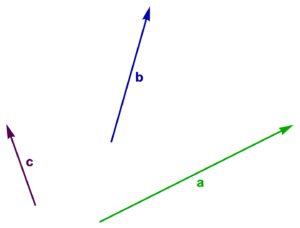
Figure 1.1 (a): Three vectors
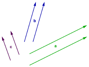
Figure 1.1 (a): Three vectors

Figure 1.1 (b): Example translations of three vectors.

Figure 1.1 (b): Example translations of three vectors.


Vector (scalar) multiplication.

We can multiply vectors by scalars by changing their lengths appropriately.

In this context a scalar is a real number (this is purposefully vague, as it will be useful to allow scalars to be complex valued later.)

Using the example vectors, some rescaled vectors include \( 2 \Ba, (-1) \Bb, \pi \Bc \), as illustrated in fig. 1.2.


Figure. 1.2 Scaled vectors.

Figure. 1.2 Scaled vectors.

Vector addition.

Scalar multiplication implicitly provides an algorithm for addition of vectors that have the same direction, as \( s \Bx + t \Bx = (s+t) \Bx \) for any scalars \( s, t \). This is illustrated in fig. 1.3 where \( 2 \Ba = \Ba + \Ba \) is formed in two equivalent forms. We see that the addition of two vectors that have the same direction requires lining up those vectors head to tail. The sum of two such vectors is the vector that can be formed from the first tail to the final head.

Figure 1.3. Twice a vector.

Figure 1.3. Twice a vector.


It turns out that this arrow daisy chaining procedure is an appropriate way of defining addition for any vectors.

Definition: Vector addition. The sum of two vectors can be found by connecting those two vectors head to tail in either order. The sum of the two vectors is the vector that can be formed by drawing an arrow from the initial tail to the final head. This can be generalized by chaining any number of vectors and joining the initial tail to the final head.

This addition procedure is illustrated in fig. 1.4, where \( \Bs = \Ba + \Bb + \Bc \) has been formed.
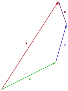
Figure 1.4. Addition of vectors.

Figure 1.4. Addition of vectors.

This definition of vector addition was inferred from the observation of the rules that must apply to addition of vectors that lay in the same direction (colinear vectors).  Is it a cheat to just declare that this rule for addition of colinear vectors also applies to arbitrary vectors?  Yes, it probably is, but it’s a cheat that works nicely, and one that models physical quantities that we experience daily (velocities, acceleration, force, …).  If you collect two friends you can demonstrate the workability of this inferred rule easily, by putting your arms out, and having your friends pull on them.  If you put your arms opposing to the sides, and have your friends pull with equal forces, you’ll see that the force that can be represented by the pulling of your friends add to zero.  If one of your friends is stronger, you’ll move more in that direction.  If you put your arms out at 45 degree angles, you’ll see that you move along the direction of the sum of the forces.  These scenarios are crudely sketched below in figure 1.x
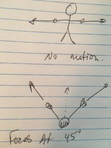
Figure 1.x: Friends pulling on your arms.

Vector subtraction.

Since we can scale a vector by \( -1 \) and we can add vectors, it is clear how to define vector subtraction

Definition: Vector subtraction. The difference of vectors \( \Ba, \Bb \) is
\begin{equation*}
\Ba – \Bb \equiv \Ba + ((-1)\Bb).
\end{equation*}

Graphically, subtracting a vector from another requires flipping the direction of the vector to be subtracted (scaling by \(-1\)), , and then adding both head to tail. This is illustrated in fig. 1.5.
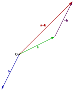
Figure 1.5. Vector subtraction.

Figure 1.5. Vector subtraction.

Length and what’s to come.

It is easy to compute the length of a vector that has an arrow representation.
One simply lines a ruler of appropriate units along the vector and measures.

We actually want an algebraic way of computing length, but there is some baggage required, including

  • Coordinates.
  • Bases (plural of basis).
  • Linear dependence and independence.
  • Dot product.
  • Metric.

The next part of this series will cover these topics. Our end goal is geometric algebra, which allows for many coordinate free operations, but we still have to use coordinates, both to read the literature, and in practice. Coordinates and non-orthonormal bases are also a good way to introduce non-Euclidean metrics.

References

[4] Vector; supervillain extraordinaire (Despicable Me). A quantity represented by an arrow with direction and magnitude. Youtube. URL https://www.youtube.com/watch?v=bOIe0DIMbI8. [Online; accessed 11-July-2020].

[Series intro] An introduction to geometric algebra.

July 25, 2020 Geometric Algebra for Electrical Engineers , , , , , , , , , , , , , , , , ,

What’s in the pipe.

It’s been a while since I did any math or physics writing. This is the first post in a series where I plan to work my way systematically from an introduction of vectors, to the axioms of geometric algebra.  I plan to start with an introduction of vectors as directed “arrows”, building on that to discuss coordinates, tuples, and column matrix representations, and representation independent ideas. With those basics established, I’ll remind the reader about how generalized vector and dot product spaces are defined and give some examples. Finally, with the foundation of vectors and vector spaces in place, I’ll introduce the concept of a multivector space, and the geometric product, and start unpacking the implications of the axioms that follow naturally from this train of thought.

The applications that I plan to include in this series will be restricted to Euclidean spaces (i.e. where length is given by the Pythagorean law), primarily those of 2 and 3 dimensions.  However, it will be good to also lay the foundations for the non-Euclidean spaces that we encounter in relativistic electromagnetism (there is actually no other kind), and in computer graphics applications of geometric algebra, especially since we can do so nearly for free.  I plan to try to introduce the requisite ideas (i.e. the metric, which allows for a generalized dot product) by discussing Euclidean non-orthonormal bases.  Such bases have applications in condensed matter physics where there are useful for modelling crystal and lattice structure, and provide a hands conceptual bridge to a set of ideas that might otherwise seem abstract and without “real world” application.

Motivation.

Many introductions to geometric algebra start by first introducing the dot product, then bivectors and the wedge product, and eventually define the product of two vectors as the synthetic sum of the dot and wedge
\begin{equation}\label{eqn:multivector:20}
\Bx \By = \Bx \cdot \By + \Bx \wedge \By.
\end{equation}
It takes a fair amount of work to do this well. In the seminal work [4] a few pages are taken for each of the dot and wedge products, showing the similarities and building up ideas, before introducing the geometric product in this fashion. In [2] the authors take a phenomenal five chapters to build up the context required to introduce the geometric product.  I am not disparaging the authors for taking that long to build up the ideas, as their introduction of the subject is exceedingly clear and thorough, and they do a lot more than the minumum required to define the geometric product.

The strategy to introduce the geometric product as a sum of dot and wedge can result in considerable confusion, especially since the wedge product is often defined in terms of the geometric product
\begin{equation}\label{eqn:multivector:40}
\Bx \wedge \By =
\inv{2} \lr{
\Bx \By – \By \Bx
}.
\end{equation}
The whole subject can appear like a chicken and egg problem. I personally found the subject very confusing initially, and had considerable difficulty understanding which of the many identities of geometric algebra were the most fundamental. For this reason, I found the axiomatic approach of [1] very refreshing. The cavaet with that work is that is is exceptionally terse, as they jammed a reformulation of most of physics using geometric algebra into that single book, and it would have been thousands of pages had they tried to make it readable by mere mortals.

When I wrote my own book on geometric algebra, I had the intuition that the way to introduce the subject ought to be like the vector space in abstract linear algebra. The construct of a vector space is a curious and indirect way to define a vector. Vectors are not defined as entities, but simply as members of a vector space, a space that is required to have a set of properties. I thought that the same approach would probably work with multivectors, which could be defined as members of a multivector space, a mathematical construction with a set of properties.

I did try this approach, but was not fully satisfied with what I wrote. I think that dissatisfaction was because I tried to define the multivector first. To define the multivector, I first introduced a whole set of prerequisite ideas (bivector, trivector, blade, k-vector, vector product, …), but that was also problematic, since the vector multiplication idea required for those concepts wasn’t fully defined until the multivector space itself was defined.

My approach shows some mathematical cowardness. Had I taken the approach of the vector space fully to heart, the multivector could have been defined as a member of a multivector space, and all the other ideas follow from that. In this multi-part series, I’m going to play with this approach anew, and see how it works out.  If it does work, I’ll see if I can incorporate this approach into a new version of my book.

Review and background.

In this series, I’m going to assume a reader interested in geometric algebra, is probably also familiar with a wide variety of concepts, including but not limited to

  • vectors,
  • coordinates,
  • matrices,
  • basis,
  • change of basis,
  • dot product,
  • real and complex numbers,
  • rotations and translations,
  • vector spaces, and
  • linear transformations.

Despite those assumptions, as mentioned above, I’m going to attempt to build up the basics of vector representation and vector spaces in a systematic fashion, starting from a very elementary level.

My reasons for doing so are mainly to explore the logical sequencing of the ideas required.  I’ve always found well crafted pedagogical sequences rewarding, and will hopefully construct one here that is appreciated by anybody who chooses to follow along.

Next time.

As preparation for the next article in this series, the reader is asked to watch a short lesson from Vector, not so supervillain extraordinaire (Despicable Me).

References

[1] C. Doran and A.N. Lasenby. Geometric algebra for physicists. Cambridge University Press New York, Cambridge, UK, 1st edition, 2003.

[2] L. Dorst, D. Fontijne, and S. Mann. Geometric Algebra for Computer Science. Morgan Kaufmann, San Francisco, 2007.

[4] D. Hestenes. New Foundations for Classical Mechanics. Kluwer Academic Publishers, 1999.

New fan and internal cleaning of my Skull canyon NUC.

July 7, 2020 electronics , , , ,

My “nuc1” has been inoperable for months, with a dead fan.  The replacement was delayed by the panic-demic significantly, but finally arrived today.  Here’s the NUC all opened up, with my replacement fan ready to be installed:


I had some trouble taking it out, and it turns out that it’s taped down, as well as screwed, so it just took some brute force.  However, check out the dust on the vents:


I’m wondering if the original fan was actually okay, and this beastie just needed a cleaning.  There wasn’t much surface area that would allow any air flow (just that tiny little corner), and I suspect that even that tiny little corner that wasn’t blocked was obscured before I pried up the old fan.

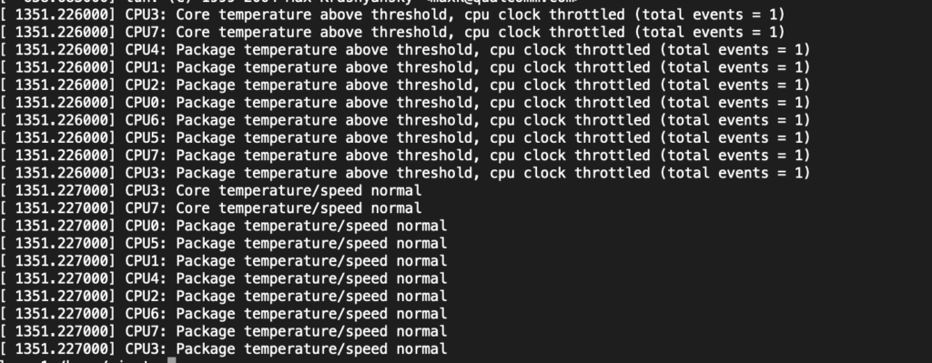
After cleaning the vents, and installing the new fan (I’d purchased it, so thought I may as well install it, even if the blocked ducts were the problem.), I can now run a parallel build without a constant barrage of temperature events.  I do get some:


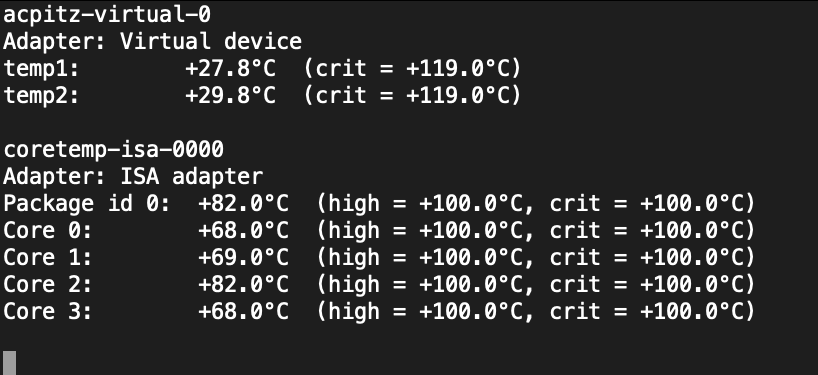
but things return to normal and the lm_sensor package (sensors program) reports core temperatures within range, despite the parallel make:

This beastie runs hot, but I already knew that.  I see the temperatures spike during make, and get near the high threshold, but not all the way there.

I’m monitoring with both dmesg -w and sensors:

#!/bin/bash

# https://unix.stackexchange.com/questions/328906/find-fan-speed-and-cpu-temp-in-linux
sudo yum install lm_sensors

while [ 0 ] ; do clear ; sensors ; sleep 5 ; done