Here’s three more fairly short Geometric Algebra related tutorials that I’ve posted on youtube
Three more geometric algebra tutorials on youtube.
January 28, 2018 math and physics play complex exponential, cross product, dot product, Geometric Algebra, line intersection, linear solution, linear system, vector product, wedge product
Electric field of a spherical shell. Ka-Tex rendered [Take II].
January 14, 2018 math and physics play KaTex, latex, MathJax, mathjax-latex, wordpress, wordpress plugin, WP-KaTex
In a previous post I attempted to use the katex plugin to render an old post instead of using Mathjax. It seems that was not actually rendered with KaTex, but (I think) it was rendered with the latex keyword handling in the Jetpack plugin, which I also had installed. I’ve customized the katex plugin I have installed to use a different keyword (katex instead of latex).
This is a test of KaTex, the latex rendering engine used for Khan academy. They advertise themselves as much faster than mathjax, but this speed comes with some usability issues.
Here’s a rerendering of an old post, with the latex rendered with WP-KaTeX instead of MathJax-LaTeX.
The post
Problem:
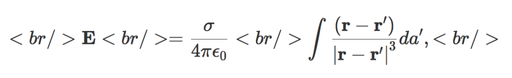
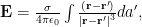
Calculate the field due to a spherical shell. The field is
[katex display=”true”]\mathbf{E} = \frac{\sigma}{4 \pi \epsilon_0} \int \frac{(\mathbf{r} – \mathbf{r}’)}{{{\left\lvert{{\mathbf{r} – \mathbf{r}’}}\right\rvert}}^3} da’,[/katex]
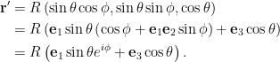
where [katex]\mathbf{r}'[/katex] is the position to the area element on the shell. For the test position, let [katex]\mathbf{r} = z \mathbf{e}_3[/katex].
Solution:
We need to parameterize the area integral. A complex-number like geometric algebra representation works nicely.
[katex display=”true”]\begin{aligned}\mathbf{r}’ &= R \left( \sin\theta \cos\phi, \sin\theta \sin\phi, \cos\theta \right) \\ &= R \left( \mathbf{e}_1 \sin\theta \left( \cos\phi + \mathbf{e}_1 \mathbf{e}_2 \sin\phi \right) + \mathbf{e}_3 \cos\theta \right) \\ &= R \left( \mathbf{e}_1 \sin\theta e^{i\phi} + \mathbf{e}_3 \cos\theta \right).\end{aligned}[/katex]
Here [katex]i = \mathbf{e}_1 \mathbf{e}_2[/katex] has been used to represent to horizontal rotation plane.
The difference in position between the test vector and area-element is
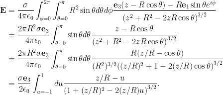
[katex display=”true”]\mathbf{r} – \mathbf{r}’ = \mathbf{e}_3 {\left({ z – R \cos\theta }\right)} – R \mathbf{e}_1 \sin\theta e^{i \phi},[/katex]
with an absolute squared length of
[katex display=”true”]\begin{aligned}{{\left\lvert{{\mathbf{r} – \mathbf{r}’ }}\right\rvert}}^2 &= {\left({ z – R \cos\theta }\right)}^2 + R^2 \sin^2\theta \\ &= z^2 + R^2 – 2 z R \cos\theta.\end{aligned}[/katex]
As a side note, this is a kind of fun way to prove the old “cosine-law” identity. With that done, the field integral can now be expressed explicitly
[katex display=”true”]\begin{aligned} \mathbf{E} &= \frac{\sigma}{4 \pi \epsilon_0} \int_{\phi = 0}^{2\pi} \int_{\theta = 0}^\pi R^2 \sin\theta d\theta d\phi \frac{\mathbf{e}_3 {\left({ z – R \cos\theta }\right)} – R \mathbf{e}_1 \sin\theta e^{i \phi}} { {\left({z^2 + R^2 – 2 z R \cos\theta}\right)}^{3/2} } \\ &= \frac{2 \pi R^2 \sigma \mathbf{e}_3}{4 \pi \epsilon_0} \int_{\theta = 0}^\pi \sin\theta d\theta \frac{z – R \cos\theta} { {\left({z^2 + R^2 – 2 z R \cos\theta}\right)}^{3/2} } \\ &= \frac{2 \pi R^2 \sigma \mathbf{e}_3}{4 \pi \epsilon_0} \int_{\theta = 0}^\pi \sin\theta d\theta \frac{ R( z/R – \cos\theta) } { (R^2)^{3/2} {\left({ (z/R)^2 + 1 – 2 (z/R) \cos\theta}\right)}^{3/2} } \\ &= \frac{\sigma \mathbf{e}_3}{2 \epsilon_0} \int_{u = -1}^{1} du \frac{ z/R – u} { {\left({1 + (z/R)^2 – 2 (z/R) u}\right)}^{3/2} }. \end{aligned}[/katex]
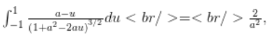
Observe that all the azimuthal contributions get killed. We expect that due to the symmetry of the problem. We are left with an integral that submits to Mathematica, but doesn’t look fun to attempt manually. Specifically
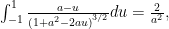
[katex display=”true”]\int_{-1}^1 \frac{a-u}{{\left({1 + a^2 – 2 a u}\right)}^{3/2}} du = \frac{2}{a^2},[/katex]
if [katex]a > 1[/katex], and zero otherwise, so
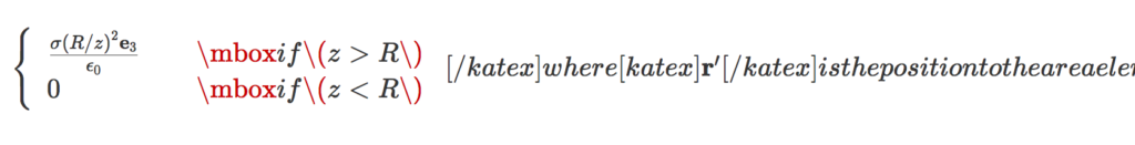
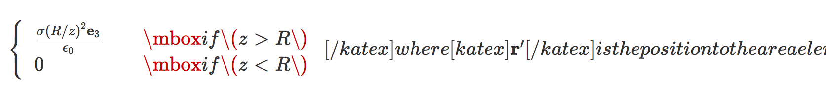
[katex display=”true”]\boxed{ \mathbf{E} = \frac{\sigma (R/z)^2 \mathbf{e}_3}{\epsilon_0} }[/katex]
for [katex]z > R[/katex], and zero otherwise.
In the problem, it is pointed out to be careful of the sign when evaluating [katex]\sqrt{ R^2 + z^2 – 2 R z }[/katex], however, I don’t see where that is even useful?
KaTex commentary
- Conditional patterns, such as:
\left\{
\begin{array}{l l}
\frac{\sigma (R/z)^2 \mathbf{e}_3}{\epsilon_0}
& \quad \mbox{if $ z > R $ } \\
0 & \quad \mbox{if $ z < R $ }
\end{array}
\right.
messed up KaTex, resulting in render errors like:

Using \( ... \) within math mode instead of $ ... $ also messed things up. Example:
\left\{
\begin{array}{l l}
\frac{\sigma (R/z)^2 \mathbf{e}_3}{\epsilon_0}
& \quad \mbox{if $ z > R $ } \\
0 & \quad \mbox{if $ z < R $ }
\end{array}
\right.
This resulted in a messed up parse like so:
It looks like it's the mbox that messes things up, and not the array itself, so \text could probably be used instead.
- The latex has to be all in one line, or else KaTex renders the newlines explicitly. Example:
Having to condense all my latex onto a single line is one of the reasons I switched from the default wordpress latex engine to mathjax. It was annoying enough that I started paying for my wordpress hosting, and stopped posting on my old free peeterjoot.wordpress.com blog. Using KaTex and having to go back to single line latex would suck!
- The rendering looks great, just like mathjax.
- The Mathjax-Latex wordpress plugin has some support for equation labeling and references. I don't see a way to do those with the WP-KaTex plugin.
- I can have a large set of macros installed in my default.js matching a subset of what I have in my .sty files. I don't see a way to do that with the WP-KaTex plugin, but perhaps there is just no documented mechanism. KaTex itself does have a macro mechanism.
- The display isn't left justified like the wordpress latex, and looks decent.

Lorentz boosts in Geometric Algebra paravector notation.
January 14, 2018 math and physics play boost, Dirac basis, Geometric Algebra, involution, lightlike, Lorentz transformation, multivector, paravector, Pauli basis, rotation, spacelike, STA, timelike
[Click here for a PDF of this post with nicer formatting]
Motivation.
The notation I prefer for relativistic geometric algebra uses Hestenes’ space time algebra (STA) [2], where the basis is a four dimensional space \( \setlr{ \gamma_\mu } \), subject to Dirac matrix like relations \( \gamma_\mu \cdot \gamma_\nu = \eta_{\mu \nu} \).
In this formalism a four vector is just the sum of the products of coordinates and basis vectors, for example, using summation convention
\begin{equation}\label{eqn:boostToParavector:160}
x = x^\mu \gamma_\mu.
\end{equation}
The invariant for a four-vector in STA is just the square of that vector
\begin{equation}\label{eqn:boostToParavector:180}
\begin{aligned}
x^2
&= (x^\mu \gamma_\mu) \cdot (x^\nu \gamma_\nu) \\
&= \sum_\mu (x^\mu)^2 (\gamma_\mu)^2 \\
&= (x^0)^2 – \sum_{k = 1}^3 (x^k)^2 \\
&= (ct)^2 – \Bx^2.
\end{aligned}
\end{equation}
Recall that a four-vector is time-like if this squared-length is positive, spacelike if negative, and light-like when zero.
Time-like projections are possible by dotting with the “lab-frame” time like basis vector \( \gamma_0 \)
\begin{equation}\label{eqn:boostToParavector:200}
ct = x \cdot \gamma_0 = x^0,
\end{equation}
and space-like projections are wedges with the same
\begin{equation}\label{eqn:boostToParavector:220}
\Bx = x \cdot \gamma_0 = x^k \sigma_k,
\end{equation}
where sums over Latin indexes \( k \in \setlr{1,2,3} \) are implied, and where the elements \( \sigma_k \)
\begin{equation}\label{eqn:boostToParavector:80}
\sigma_k = \gamma_k \gamma_0.
\end{equation}
which are bivectors in STA, can be viewed as an Euclidean vector basis \( \setlr{ \sigma_k } \).
Rotations in STA involve exponentials of space like bivectors \( \theta = a_{ij} \gamma_i \wedge \gamma_j \)
\begin{equation}\label{eqn:boostToParavector:240}
x’ = e^{ \theta/2 } x e^{ -\theta/2 }.
\end{equation}
Boosts, on the other hand, have exactly the same form, but the exponentials are with respect to space-time bivectors arguments, such as \( \theta = a \wedge \gamma_0 \), where \( a \) is any four-vector.
Observe that both boosts and rotations necessarily conserve the space-time length of a four vector (or any multivector with a scalar square).
\begin{equation}\label{eqn:boostToParavector:260}
\begin{aligned}
\lr{x’}^2
&=
\lr{ e^{ \theta/2 } x e^{ -\theta/2 } } \lr{ e^{ \theta/2 } x e^{ -\theta/2 } } \\
&=
e^{ \theta/2 } x \lr{ e^{ -\theta/2 } e^{ \theta/2 } } x e^{ -\theta/2 } \\
&=
e^{ \theta/2 } x^2 e^{ -\theta/2 } \\
&=
x^2 e^{ \theta/2 } e^{ -\theta/2 } \\
&=
x^2.
\end{aligned}
\end{equation}
Paravectors.
Paravectors, as used by Baylis [1], represent four-vectors using a Euclidean multivector basis \( \setlr{ \Be_\mu } \), where \( \Be_0 = 1 \). The conversion between STA and paravector notation requires only multiplication with the timelike basis vector for the lab frame \( \gamma_0 \)
\begin{equation}\label{eqn:boostToParavector:40}
\begin{aligned}
X
&= x \gamma_0 \\
&= \lr{ x^0 \gamma_0 + x^k \gamma_k } \gamma_0 \\
&= x^0 + x^k \gamma_k \gamma_0 \\
&= x^0 + \Bx \\
&= c t + \Bx,
\end{aligned}
\end{equation}
We need a different structure for the invariant length in paravector form. That invariant length is
\begin{equation}\label{eqn:boostToParavector:280}
\begin{aligned}
x^2
&=
\lr{ \lr{ ct + \Bx } \gamma_0 }
\lr{ \lr{ ct + \Bx } \gamma_0 } \\
&=
\lr{ \lr{ ct + \Bx } \gamma_0 }
\lr{ \gamma_0 \lr{ ct – \Bx } } \\
&=
\lr{ ct + \Bx }
\lr{ ct – \Bx }.
\end{aligned}
\end{equation}
Baylis introduces an involution operator \( \overline{{M}} \) which toggles the sign of any vector or bivector grades of a multivector. For example, if \( M = a + \Ba + I \Bb + I c \), where \( a,c \in \mathbb{R} \) and \( \Ba, \Bb \in \mathbb{R}^3 \) is a multivector with all grades \( 0,1,2,3 \), then the involution of \( M \) is
\begin{equation}\label{eqn:boostToParavector:300}
\overline{{M}} = a – \Ba – I \Bb + I c.
\end{equation}
Utilizing this operator, the invariant length for a paravector \( X \) is \( X \overline{{X}} \).
Let’s consider how boosts and rotations can be expressed in the paravector form. The half angle operator for a boost along the spacelike \( \Bv = v \vcap \) direction has the form
\begin{equation}\label{eqn:boostToParavector:120}
L = e^{ -\vcap \phi/2 },
\end{equation}
\begin{equation}\label{eqn:boostToParavector:140}
\begin{aligned}
X’
&=
c t’ + \Bx’ \\
&=
x’ \gamma_0 \\
&=
L x L^\dagger \\
&=
e^{ -\vcap \phi/2 } x^\mu \gamma_\mu
e^{ \vcap \phi/2 } \gamma_0 \\
&=
e^{ -\vcap \phi/2 } x^\mu \gamma_\mu \gamma_0
e^{ -\vcap \phi/2 } \\
&=
e^{ -\vcap \phi/2 } \lr{ x^0 + \Bx } e^{ -\vcap \phi/2 } \\
&=
L X L.
\end{aligned}
\end{equation}
Because the involution operator toggles the sign of vector grades, it is easy to see that the required invariance is maintained
\begin{equation}\label{eqn:boostToParavector:320}
\begin{aligned}
X’ \overline{{X’}}
&=
L X L
\overline{{ L X L }} \\
&=
L X L
\overline{{ L }} \overline{{ X }} \overline{{ L }} \\
&=
L X \overline{{ X }} \overline{{ L }} \\
&=
X \overline{{ X }} L \overline{{ L }} \\
&=
X \overline{{ X }}.
\end{aligned}
\end{equation}
Let’s explicitly expand the transformation of \ref{eqn:boostToParavector:140}, so we can relate the rapidity angle \( \phi \) to the magnitude of the velocity. This is most easily done by splitting the spacelike component \( \Bx \) of the four vector into its projective and rejective components
\begin{equation}\label{eqn:boostToParavector:340}
\begin{aligned}
\Bx
&= \vcap \vcap \Bx \\
&= \vcap \lr{ \vcap \cdot \Bx + \vcap \wedge \Bx } \\
&= \vcap \lr{ \vcap \cdot \Bx } + \vcap \lr{ \vcap \wedge \Bx } \\
&= \Bx_\parallel + \Bx_\perp.
\end{aligned}
\end{equation}
The exponential
\begin{equation}\label{eqn:boostToParavector:360}
e^{-\vcap \phi/2}
=
\cosh\lr{ \phi/2 }
– \vcap \sinh\lr{ \phi/2 },
\end{equation}
commutes with any scalar grades and with \( \Bx_\parallel \), but anticommutes with \( \Bx_\perp \), so
\begin{equation}\label{eqn:boostToParavector:380}
\begin{aligned}
X’
&=
\lr{ c t + \Bx_\parallel } e^{ -\vcap \phi/2 } e^{ -\vcap \phi/2 }
+
\Bx_\perp e^{ \vcap \phi/2 } e^{ -\vcap \phi/2 } \\
&=
\lr{ c t + \Bx_\parallel } e^{ -\vcap \phi }
+
\Bx_\perp \\
&=
\lr{ c t + \vcap \lr{ \vcap \cdot \Bx } } \lr{ \cosh \phi – \vcap \sinh \phi }
+
\Bx_\perp \\
&=
\Bx_\perp
+
\lr{ c t \cosh\phi – \lr{ \vcap \cdot \Bx} \sinh \phi }
+
\vcap \lr{ \lr{ \vcap \cdot \Bx } \cosh\phi – c t \sinh \phi } \\
&=
\Bx_\perp
+
\cosh\phi \lr{ c t – \lr{ \vcap \cdot \Bx} \tanh \phi }
+
\vcap \cosh\phi \lr{ \vcap \cdot \Bx – c t \tanh \phi }.
\end{aligned}
\end{equation}
Employing the argument from [3],
we want \( \phi \) defined so that this has structure of a Galilean transformation in the limit where \( \phi \rightarrow 0 \). This means we equate
\begin{equation}\label{eqn:boostToParavector:400}
\tanh \phi = \frac{v}{c},
\end{equation}
so that for small \(\phi\)
\begin{equation}\label{eqn:boostToParavector:420}
\Bx’ = \Bx – \Bv t.
\end{equation}
We can solving for \( \sinh^2 \phi \) and \( \cosh^2 \phi \) in terms of \( v/c \) using
\begin{equation}\label{eqn:boostToParavector:440}
\tanh^2 \phi
= \frac{v^2}{c^2}
=
\frac{ \sinh^2 \phi }{1 + \sinh^2 \phi}
=
\frac{ \cosh^2 \phi – 1 }{\cosh^2 \phi}.
\end{equation}
which after picking the positive root required for Galilean equivalence gives
\begin{equation}\label{eqn:boostToParavector:460}
\begin{aligned}
\cosh \phi &= \frac{1}{\sqrt{1 – (\Bv/c)^2}} \equiv \gamma \\
\sinh \phi &= \frac{v/c}{\sqrt{1 – (\Bv/c)^2}} = \gamma v/c.
\end{aligned}
\end{equation}
The Lorentz boost, written out in full is
\begin{equation}\label{eqn:boostToParavector:480}
ct’ + \Bx’
=
\Bx_\perp
+
\gamma \lr{ c t – \frac{\Bv}{c} \cdot \Bx }
+
\gamma \lr{ \vcap \lr{ \vcap \cdot \Bx } – \Bv t }
.
\end{equation}
Authors like Chappelle, et al., that also use paravectors [4], specify the form of the Lorentz transformation for the electromagnetic field, but for that transformation reversion is used instead of involution.
I plan to explore that in a later post, starting from the STA formalism that I already understand, and see if I can make sense
of the underlying rationale.
References
[1] William Baylis. Electrodynamics: a modern geometric approach, volume 17. Springer Science \& Business Media, 2004.
[2] C. Doran and A.N. Lasenby. Geometric algebra for physicists. Cambridge University Press New York, Cambridge, UK, 1st edition, 2003.
[3] L. Landau and E. Lifshitz. The Classical theory of fields. Addison-Wesley, 1951.
[4] James M Chappell, Samuel P Drake, Cameron L Seidel, Lachlan J Gunn, and Derek Abbott. Geometric algebra for electrical and electronic engineers. Proceedings of the IEEE, 102 0(9), 2014.
Electric field of a spherical shell. Ka-Tex rendered
January 10, 2018 math and physics play KaTex, latex, MathJax, mathjax-latex, wordpress, wordpress plugin, WP-KaTex
This is a test of KaTex, the latex rendering engine used for Khan academy. They advertise themselves as much faster than mathjax, but it looks like the reason for that is because they generate images that look crappy unless the browser resolution is matched to the images just right.
Here’s a rerendering of an old post, with the latex rendered with WP-KaTeX instead of MathJax-LaTeX.
The post
Problem:
Calculate the field due to a spherical shell. The field is
where 

Solution:
We need to parameterize the area integral. A complex-number like geometric algebra representation works nicely.
Here 
The difference in position between the test vector and area-element is

with an absolute squared length of

As a side note, this is a kind of fun way to prove the old “cosine-law” identity. With that done, the field integral can now be expressed explicitly
Observe that all the azimuthal contributions get killed. We expect that due to the symmetry of the problem. We are left with an integral that submits to Mathematica, but doesn’t look fun to attempt manually. Specifically
if 

for 
In the problem, it is pointed out to be careful of the sign when evaluating 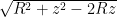
KaTex commentary
- Conditional patterns, such as:
\left\{
\begin{array}{l l}
\frac{\sigma (R/z)^2 \mathbf{e}_3}{\epsilon_0}
& \quad \mbox{if \( z > R \) } \\
0 & \quad \mbox{if \( z < R \) }
\end{array}
\right.
messed up KaTex, resulting in render errors like:

- The latex has to be all in one line, or else KaTex renders the newlines explicitly. Example:
 Having to condense all my latex onto a single line is one of the reasons I switched from the default wordpress latex engine to mathjax. It was annoying enough that I started paying for my wordpress hosting, and stopped posting on my old free peeterjoot.wordpress.com blog. Using KaTex and having to go back to single line latex would suck!
 - The rendering looks like crap, unless you match your resolution to exactly those used to create the images. The mathjax rendering may be slower, but looks much better!
- The Mathjax-Latex wordpress plugin has some support for equation labeling and references. I don’t see a way to do those with the WP-KaTex plugin.
- I can have a large set of macros installed in my default.js matching a subset of what I have in my .sty files. I don’t see a way to do that with the WP-KaTex plugin, but perhaps there is just no documented mechanism. KaTex itself does have a macro mechanism.
- Left justified display mode is hard to read. The mathjax rendered centered display mode looks much better.
EDIT.
I’m not sure I was getting the katex plugin when I used the [ latex ] … [ /latex ] tags. I see some comments that indicate that there is built in handling of these tags in the Jetpack plugin. If I change frontend.php in the katex plugin to use [ katex ] … [ /katex ] tags instead, then I see much different results.
Christmas gift from Lance: some assembly required
December 25, 2017 Incoherent ramblings ASCII, Christmas
Lance got me a little notebook for Christmas, the first page of which had a message that I had to work to decode:
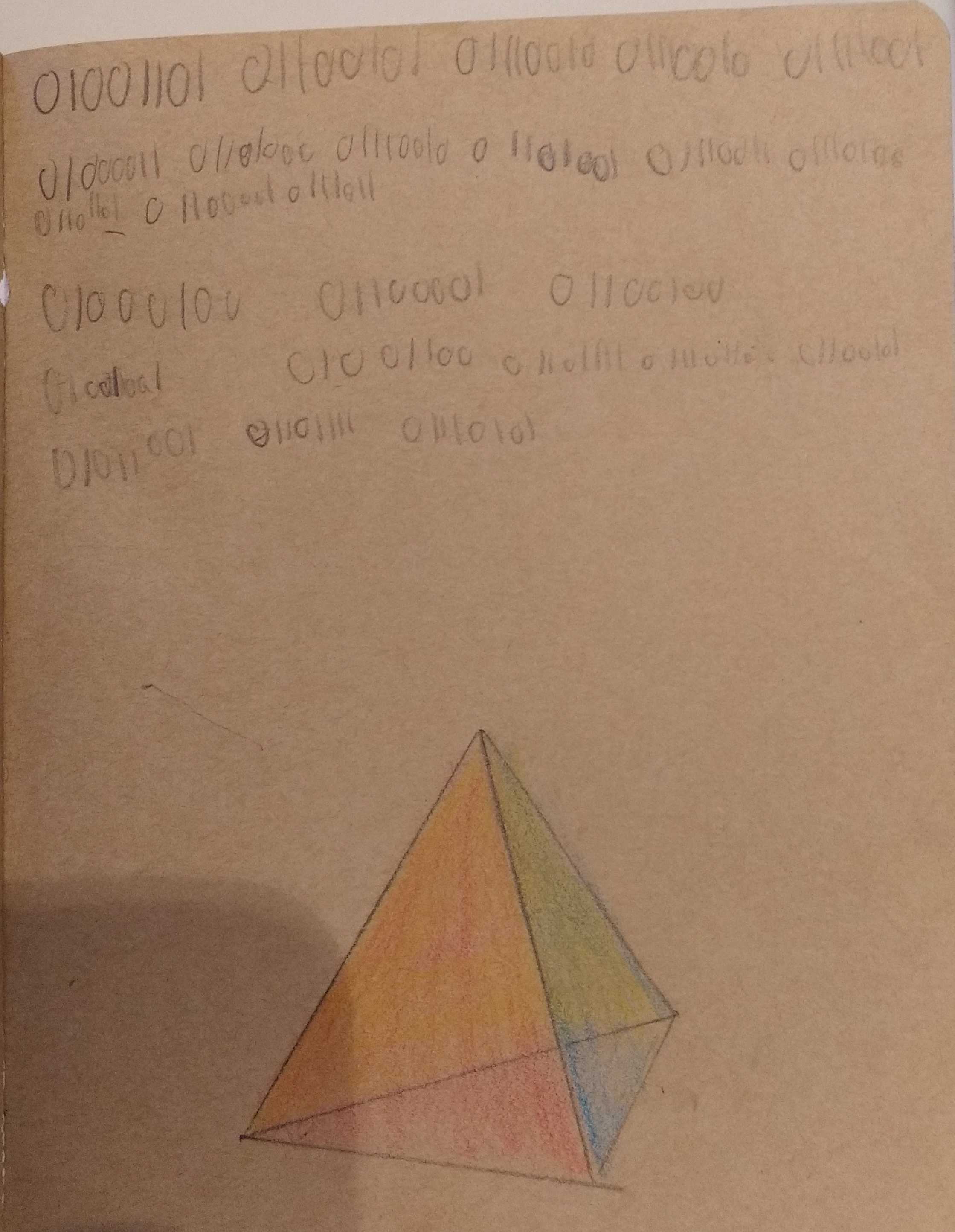
Conveniently, it was all ASCII, and all in a single base. He got the evil idea of wishing he’d encoding each character in a different base, which would have made life more difficult. I used the following quick hack to decode:
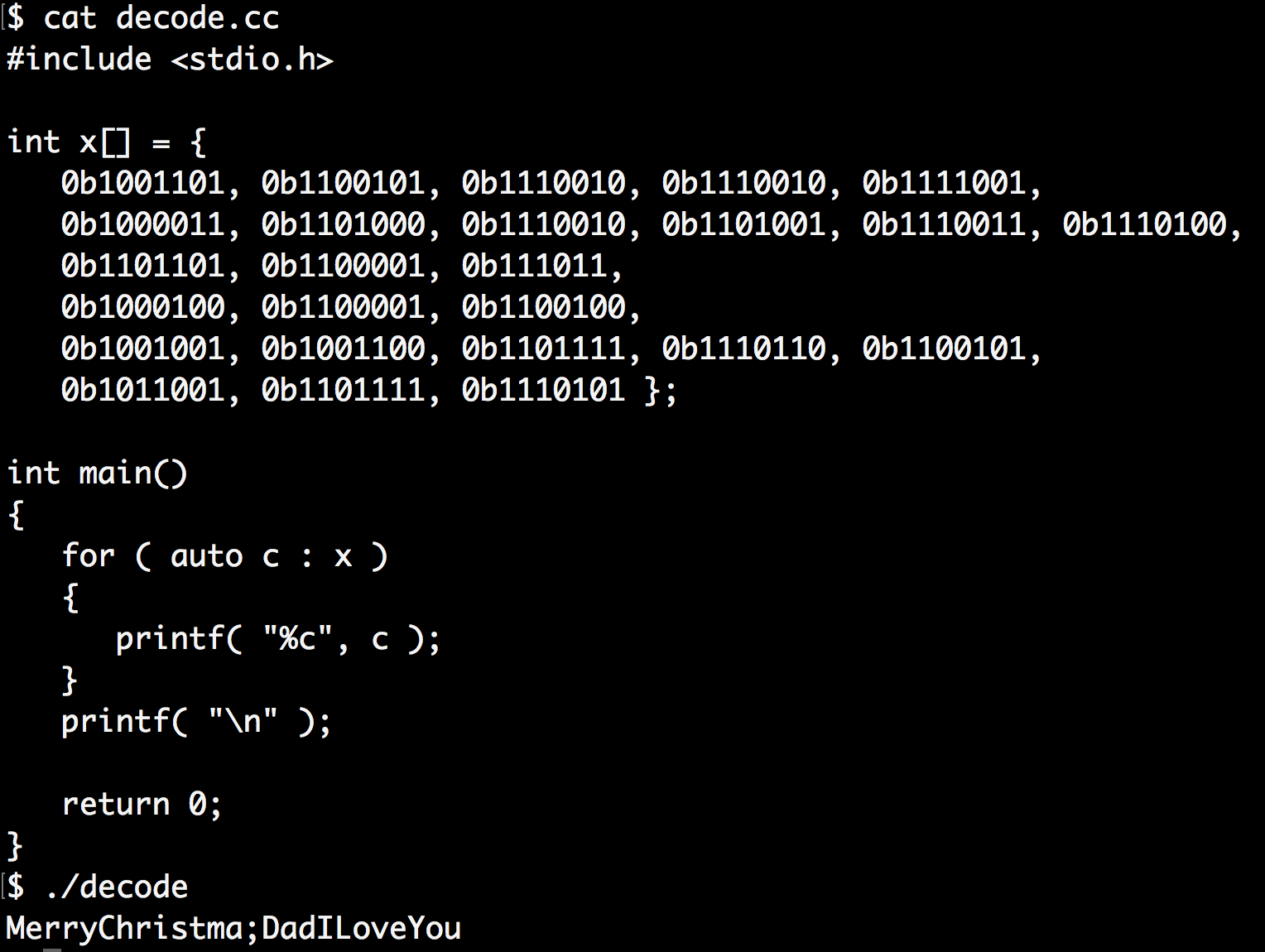
There was one small encoding error, a missing zero that transformed an ‘s’ into a ‘;’.