integral

A PV integral using contour integration.

January 27, 2025 math and physics play , , , , , ,

[Click here for a PDF version of this post]

Here’s the second last real-integral sub-problem from [1], problem 31(j). Find
\begin{equation}\label{eqn:oscillatorKernel:20}
I = P \int_{-\infty}^\infty \inv{ \lr{ \omega’ – \omega_0 }^2 + a^2 } \inv{ \omega’ – \omega } d\omega’.
\end{equation}

Our poles are sitting at \( \omega \), and
\begin{equation}\label{eqn:oscillatorKernel:80}
\alpha, \beta = \omega_0 \pm i a
\end{equation}
one of which sits above the x-axis, one below, and one on the line.

This means that if we compute the usual infinite semicircular contour integral, we have a \( 2 \pi i \) weighted residue above the line and one \( \pi i \) weighted residue for the x-axis pole. That is
\begin{equation}\label{eqn:oscillatorKernel:50}
\begin{aligned}
\oint \inv{ \lr{ z – \omega_0 }^2 + a^2 } \inv{ z – \omega } dz
&=
\lr{ 2 \pi i } \evalbar{ \inv{\lr{z – \lr{ \omega_0 – i a } } \lr{ z – \omega } } }{z = \omega_0 + i a }
+
\lr{ \pi i } \evalbar{ \inv{ \lr{ z – \omega_0 }^2 + a^2 }}{z = \omega } \\
&=
\lr{ 2 \pi i } \inv{\lr{\omega_0 + i a – \lr{ \omega_0 – i a } } \lr{ \omega_0 + i a – \omega } }
+
\lr{ \pi i } \inv{ \lr{ \omega – \omega_0 }^2 + a^2 } \\
&=
\frac{ 2 \pi i }{2 i a} \inv{ \omega_0 + i a – \omega } \frac{ \omega_0 – i a – \omega }{\omega_0 – i a – \omega }
+
\lr{ \pi i } \inv{ \lr{ \omega – \omega_0 }^2 + a^2 } \\
&=
\frac{ \pi }{ \lr{ \omega – \omega_0 }^2 + a^2 } \lr{ \frac{\omega_0 – \omega}{a} – i + i },
\end{aligned}
\end{equation}
or
\begin{equation}\label{eqn:oscillatorKernel:100}
\boxed{
I =
\frac{ \pi \lr{ \omega_0 – \omega } }{ a \lr{ \lr{ \omega – \omega_0 }^2 + a^2} }.
}
\end{equation}

Interestingly, Mathematica doesn’t seem to be able to solve this integral, even setting PrincipleValue to True. The solution ends up with a bogus seeming \( \textrm{Im}\left(\omega_0-\omega \right) = \textrm{Re}(a) \) restriction, and as far as I can tell, the Mathematica result is also zero after simplification that it fails to do. Mathematica can solve this if we explicitly state the PV condition as a limit, as shown in fig. 1.

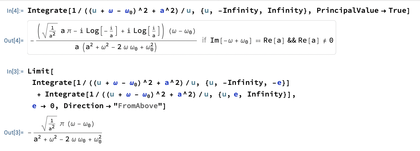
fig. 1. Coercing Mathematica to evaluate this.

References

[1] F.W. Byron and R.W. Fuller. Mathematics of Classical and Quantum Physics. Dover Publications, 1992.

A fun ellipse related integral.

January 18, 2025 math and physics play , , ,

[Click here for a PDF version of this post]

Motivation.

This was a problem I found on twitter ([2])

Find
\begin{equation}\label{eqn:ellipicalIntegral:20}
I = \int_0^\pi \frac{dx}{a^2 \cos^2 x + b^2 \sin^2 x}.
\end{equation}

I posted my solution there (as a screenshot), but had a sign wrong. Here’s a correction.

Solution.

Let’s first assume we aren’t interested in the \( a^2 = b^2 \), nor either of the \( a = 0, b = 0\) cases (if either of \( a, b \) is zero, then the integral is divergent.)

We can make a couple simple transformations to start with
\begin{equation}\label{eqn:ellipicalIntegral:40}
\begin{aligned}
\cos^2 x &= \frac{\cos(2x) + 1}{2} \\
\sin^2 x &= \frac{1 – \cos(2x)}{2},
\end{aligned}
\end{equation}
and then \( u = 2 x \), for \( dx = du/2 \)
\begin{equation}\label{eqn:ellipicalIntegral:60}
\begin{aligned}
I
&= \int_0^{2\pi} 2 \frac{du/2}{a^2 \lr{ 1 + \cos u } + b^2 \lr{1 – \cos u}} \\
&= \int_0^{2\pi} \frac{du}{ \lr{ a^2 – b^2 } \cos u + a^2 + b^2 }.
\end{aligned}
\end{equation}
There is probably a simple way to evaluate this integral, but let’s try it the fun way, using contour integration. Following examples from [1], let \( z = e^{i u} \), where \( dz = i z du \), and \( \alpha = \lr{ a^2 + b^2 }/\lr{ a^2 – b^2 } \), for
\begin{equation}\label{eqn:ellipicalIntegral:80}
\begin{aligned}
I
&= \oint_{\Abs{z} = 1} \frac{dz/(i z)}{ \lr{ a^2 – b^2 } \lr{ z + \inv{z}}/2 + a^2 + b^2 } \\
&= \frac{2}{i \lr{ a^2 – b^2 }} \oint_{\Abs{z} = 1} \frac{dz}{ z \lr{ z + \inv{z} + 2 \alpha} } \\
&= \frac{2}{i \lr{ a^2 – b^2 }} \oint_{\Abs{z} = 1} \frac{dz}{ z^2 + 2 \alpha z + 1 } \\
&= \frac{2}{i \lr{ a^2 – b^2 }} \oint_{\Abs{z} = 1} \frac{dz}{ \lr{ z + \alpha – \sqrt{\alpha^2 – 1}}\lr{ z + \alpha + \sqrt{\alpha^2 – 1}} }.
\end{aligned}
\end{equation}

There is a single enclosed pole on the real axis. For \( a^2 > b^2 \) where \( \alpha > 0 \) that pole is at \( z = -\alpha + \sqrt{ \alpha^2 – 1} \), so the integral is
\begin{equation}\label{eqn:ellipicalIntegral:100}
\begin{aligned}
I
&= 2 \pi i \frac{2}{i \lr{ a^2 – b^2 }} \evalbar{ \frac{1}{ z + \alpha + \sqrt{\alpha^2 – 1 } }}{z = -\alpha + \sqrt{ \alpha^2 – 1}} \\
&= \frac{4 \pi}{ a^2 – b^2 } \frac{1}{ 2 \sqrt{\alpha^2 – 1 } } \\
&= \frac{4 \pi }{ 2 \sqrt{\lr{a^2 + b^2}^2 – \lr{a^2 – b^2}^2 } } \\
&= \frac{2 \pi }{ \sqrt{4 a^2 b^2 } } \\
&= \frac{\pi }{ \Abs{ a b } },
\end{aligned}
\end{equation}
and for \( a^2 < b^2 \) where \( \alpha < 0 \), the enclosed pole is at \( z = -\alpha – \sqrt{ \alpha^2 – 1} \), where
\begin{equation}\label{eqn:ellipicalIntegral:120}
\begin{aligned}
I
&= 2 \pi i \frac{2}{i \lr{ a^2 – b^2 }} \evalbar{ \frac{1}{ z + \alpha – \sqrt{\alpha^2 – 1 } }}{z = -\alpha – \sqrt{ \alpha^2 – 1}} \\
&= \frac{4 \pi}{ a^2 – b^2 } \frac{1}{ -2 \sqrt{\alpha^2 – 1 } } \\
&= \frac{4 \pi}{ b^2 – a^2 } \frac{1}{ 2 \sqrt{\alpha^2 – 1 } } \\
&= \frac{4 \pi }{ 2 \sqrt{\lr{a^2 + b^2}^2 – \lr{b^2 – a^2}^2 } } \\
&= \frac{2 \pi }{ \sqrt{4 a^2 b^2 } } \\
&= \frac{\pi }{ \Abs{ a b } }.
\end{aligned}
\end{equation}
Observe that this also holds for the \( a = b \) case.

References

[1] F.W. Byron and R.W. Fuller. Mathematics of Classical and Quantum Physics. Dover Publications, 1992.

[2] CalcInsights. A decent integral problem to try out, 2025. URL https://x.com/CalcInsights_/status/1880110549146431780. [Online; accessed 18-Jan-2025].