Mathematica

Weighted geometric series

March 23, 2025 math and physics play , , ,

[Click here for a PDF version of this post]

Karl needed to evaluate the sum:

\begin{equation}\label{eqn:weightedGeometric:20}
S = \sum_{k = 0}^9 \frac{a + b k}{\lr{ 1 + i }^k}
\end{equation}

He ended up using a spreadsheet, which was a quick and effective way to deal with the problem. I was curious about this sum, since he asked me how to sum it symbolically, and I didn’t know.

Mathematica doesn’t have any problem with it, as seen in fig. 1.

fig. 1. A funky sum.

How can we figure this out?

Let’s write \( r = 1/(1+i) \) to start with, and break up the sum into constituent parts
\begin{equation}\label{eqn:weightedGeometric:40}
\begin{aligned}
S_n
&= \sum_{k = 0}^n \frac{a + b k}{\lr{ 1 + i }^k} \\
&= a \sum_{k = 0}^n r^k + b \sum_{k = 0}^n k r^k.
\end{aligned}
\end{equation}
We can evaluate the geometric part of this easily using the usual trick. Let
\begin{equation}\label{eqn:weightedGeometric:60}
T_n = \sum_{k = 0}^n r^k,
\end{equation}
then
\begin{equation}\label{eqn:weightedGeometric:80}
r T_n – T_n = r^{n+1} – 1,
\end{equation}
so
\begin{equation}\label{eqn:weightedGeometric:100}
T_n = \frac{r^{n+1} – 1}{r – 1}.
\end{equation}
Now we just have to figure out how to sum
\begin{equation}\label{eqn:weightedGeometric:120}
G_n = \sum_{k = 0}^n k r^k = \sum_{k = 1}^n k r^k.
\end{equation}
This looks suspiciously like the derivative of a geometric series. Let’s evaluate such a derivative, as a function of r:
\begin{equation}\label{eqn:weightedGeometric:140}
\begin{aligned}
\frac{d T_n(r)}{dr}
&= \sum_{k = 0}^n \frac{d}{dr} r^k \\
&= \sum_{k = 0}^n k r^{k-1} \\
&= \sum_{k = 1}^n k r^{k-1} \\
&= \inv{r} \sum_{k = 1}^n k r^k.
\end{aligned}
\end{equation}
Having summed the geometric series, we may also take the derivative of that summed result
\begin{equation}\label{eqn:weightedGeometric:160}
\begin{aligned}
\frac{d T_n(r)}{dr}
&= \frac{d}{dr} \lr{ \frac{r^{n+1} – 1}{r – 1} } \\
&= \frac{(n+1)r^n}{r – 1} – \frac{r^{n+1} – 1}{\lr{r -1}^2} \\
&= \frac{(n+1)r^n(r-1) – \lr{r^{n+1} – 1}}{\lr{r -1}^2}.
\end{aligned}
\end{equation}
Putting the pieces together, we have
\begin{equation}\label{eqn:weightedGeometric:180}
T_n = \frac{r}{\lr{r -1}^2} \lr{ (n+1)r^n(r-1) – \lr{r^{n+1} – 1} }.
\end{equation}

This means that our sum is
\begin{equation}\label{eqn:weightedGeometric:200}
S_n = a \frac{r^{n+1} – 1}{r – 1} + b \frac{r}{\lr{r -1}^2} \lr{ (n+1)r^n(r-1) – \lr{r^{n+1} – 1} }.
\end{equation}
Putting back \( r = 1/(1+i) \), and subsequent simplification, gives the Mathematica result. It’s not pretty, but at least we can do it if we want to.

Shout out to Grok that pointed out the derivative trick for the second series.  I’d forgotten that one.

Using chatgpt as online Mathematica help

January 26, 2024 Mathematica , , , ,

Here is a question that I probably would have posed at mathematica.stackexchange.com in the past, but this time I tried it using ChatGPT

“In Mathematica, I can sort by the last element in a list using something like:

SortBy[{{1, 2, 3}, {2, 3, 1}, {3, 1, 2}}, Last]

How do I specify two sort keys, for example, sort using Last as the primary key, and First as a secondary key?”


Turns out that the answer was in the Mathematica help too, right in the synopsis:


but I didn’t see it, since I’d gone straight to the examples, and didn’t see anything there.

ChatGPT should have a fun mode like Grok.  The obvious answer should have made fun of my sample query, cut and pasted from the Mathematica SortBy help, perhaps:

“Your example sucks, since sorting by the primary key is sufficient.  If you really want to waste computing cycles, this is how to do what you asked…”

My real Sort was:

filtered3 = SortBy[Select[raw3, ( (# // Last) > 0 ) &], {Last, First}];

to produce the following table of router bushing offsets + bit size:

The sort for that table did require a primary and secondary key, and initially didn’t have a nice ordering.

Updated figures in ‘Geometric Algebra for Electrical Engineers’

September 2, 2023 Geometric Algebra for Electrical Engineers , , ,

New version of the book is now published (online PDF and leanpub versions updated, with amazon updates in the approval pipeline)

  • V0.1.19-2 (Sep 2, 2023)
    • Reworked many of the Mathematica generated figures.  Now using the MaTeX[] extension to do the figure labelling (that was only done in a couple figures before this), as it looks much better, and is consistent with the fonts in the text.

      Each of these are individually very small changes, barely noticeable, but I think it makes a nice difference to overall quality.

      In many cases, I’ve generated new separate figures for the amazon paper editions of the book, using straight black instead of colors, so they don’t look as washed out, after conversion to black and white.

Here’s an example where just the captioning was changed:

The font is now whatever LaTeX uses for \\mathbf{n}, so it matches the text.

I think that the new Mathematica version (13.2) that I am using, also happens to render this 3D figure a bit nicer.

Here’s a comparison of one of the figures that now has a black and white specialization (old, new-color, new-bw):

In this particular case, I chose not to color the labels like I did previously, but I have retained that label color matching in some places.

Like I said, it’s a small difference, but the latex labelling just look better, period.  Notice that the numeric values at the tick marks on the border of the figure are not using a matching font (those are directly generated by Mathematica).  I’ll have to figure out how to make those use MaTeX too, and audit all the figures for that, but that’s a game for another day.

Inscribed Triangle in circle problem

December 25, 2022 math and physics play , , , , , ,

[Click here for a PDF version of this post]

In the LinkedIn Pre-University Geometric Algebra group, James presents a problem from the MindYourDecisions youtube channel Impossible Viral Problem, as a candidate for solution using geometric algebra.

I tried this out and found a couple ways to solve it. One of those I’ll detail here. I have to admit that part of the reason that I wanted to solve this is that the figure in the beginning of the video really bugged me. The triangle that was inscribed in the circle didn’t have any of the length properties from the problem. I could do much better with a sloppy freehand sketch, but to do a good figure, you have to actually solve for the vertexes of the triangle (once you do that, the area is easy to figure out.)

Formulating the problem.

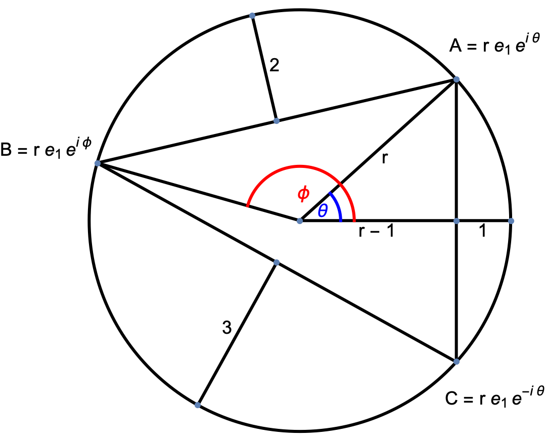
Having solved the problem, the geometry of the problem is illustrated in fig. 1.

fig. 1. Inscribed triangle in circle.

fig. 1. Inscribed triangle in circle.

I set up the problem so that the \( A,C \) triangle vertices were symmetric with respect to the x-axis, and the \(B \) vertex located elsewhere. I can describe those algebraically as
\begin{equation}\label{eqn:inscribedTriangleProblem:20}
\begin{aligned}
\BA &= r \Be_1 e^{i\theta} \\
\BC &= r \Be_1 e^{-i\theta} \\
\BB &= r \Be_1 e^{i\phi},
\end{aligned}
\end{equation}
where the radius \( r \) and two angles \( \theta, \phi \) are to be determined, and \( i = \Be_1 \Be_1\) the pseudoscalar for the \(x-y\) plane.
The vector pointing to the midpoint of the upper triangular face is given by the average of the \( \BA, \BB \) vectors, which can be seen from
\begin{equation}\label{eqn:inscribedTriangleProblem:40}
\BA + \frac{\BB – \BA}{2} = \frac{\BA + \BB}{2},
\end{equation}
and similarly, the midpoint of the lower face is found at
\begin{equation}\label{eqn:inscribedTriangleProblem:60}
\BC + \frac{\BB – \BC}{2} = \frac{\BB + \BC}{2},
\end{equation}
The problem tells us that the respective lengths of those vectors from the origin are \( r-2, r – 3\) respectively, so
\begin{equation}\label{eqn:inscribedTriangleProblem:80}
\begin{aligned}
r – 2 &= \inv{2} \Abs{ \BA + \BB } \\
r – 3 &= \inv{2} \Abs{ \BB + \BC },
\end{aligned}
\end{equation}
or
\begin{equation}\label{eqn:inscribedTriangleProblem:100}
\begin{aligned}
(r – 2)^2 &= \frac{r^2}{4} \lr{ \Be_1 e^{i\theta} + \Be_1 e^{i\phi} }^2 \\
(r – 3)^2 &= \frac{r^2}{4} \lr{ \Be_1 e^{i\phi} + \Be_1 e^{-i\theta} }^2 \\
\end{aligned}
\end{equation}
Finally, since the midpoint of the right edge is found at \( (r-1)\Be_1 \), it is clear that
\begin{equation}\label{eqn:inscribedTriangleProblem:120}
\frac{r-1}{r} = \cos\theta,
\end{equation}
or
\begin{equation}\label{eqn:inscribedTriangleProblem:140}
r = \inv{1 – \cos\theta}.
\end{equation}
This leaves us with three equations and three unknowns. Unfortunately, these are rather non-linear equations. In the video, a direct method of solving equivalent equations was demonstrated, but I picked the lazy route, and used Mathematica’s NSolve routine, solving for \( r,\theta, \phi\) numerically. Since NSolve has intrinsic complex number support, I made the following substitutions:
\begin{equation}\label{eqn:inscribedTriangleProblem:160}
\begin{aligned}
z &= e^{i\theta} \\
w &= e^{i\phi},
\end{aligned}
\end{equation}
and then plugged those into our relations above, after expanding the squares, to find
\begin{equation}\label{eqn:inscribedTriangleProblem:180}
\begin{aligned}
\lr{ \Be_1 e^{i\theta} + \Be_1 e^{i\phi} }^2
&=
2 + \Be_1 e^{i\theta} \Be_1 e^{i\phi} + \Be_1 e^{i\phi} \Be_1 e^{i\theta} \\
&=
2 + e^{-i\theta} \Be_1^2 e^{i\phi} + e^{-i\phi} \Be_1^2 e^{i\theta} \\
&=
2 + e^{-i\theta} \Be_1^2 e^{i\phi} + e^{-i\phi} \Be_1^2 e^{i\theta} \\
&=
2 + \frac{w}{z} + \frac{z}{w},
\end{aligned}
\end{equation}
and
\begin{equation}\label{eqn:inscribedTriangleProblem:200}
\begin{aligned}
\lr{ \Be_1 e^{i\phi} + \Be_1 e^{-i\theta} }^2
&=
2 + \Be_1 e^{i\phi} \Be_1 e^{-i\theta} + \Be_1 e^{-i\theta} \Be_1 e^{i\phi} \\
&=
2 + e^{-i\phi} e^{-i\theta} + e^{ i\theta} e^{i\phi} \\
&=
2 + w z + \inv{w z}.
\end{aligned}
\end{equation}
This gives us
\begin{equation}\label{eqn:inscribedTriangleProblem:220}
\begin{aligned}
4 \lr{ \frac{r – 2 }{r} }^2 &= 2 + \frac{w}{z} + \frac{z}{w} \\
4 \lr{ \frac{r – 3 }{r} }^2 &= 2 + w z + \inv{w z},
\end{aligned}
\end{equation}
where
\begin{equation}\label{eqn:inscribedTriangleProblem:240}
r = \inv{1 – \inv{2}\lr{ z + \inv{z}}}.
\end{equation}

The NSolve gave me some garbage solutions (like \(\theta = 0 \)) that must have been valid numerically, but did not encode the geometry of the problem, so I added a few additional constraints to the problem, namely
\begin{equation}\label{eqn:inscribedTriangleProblem:260}
\begin{aligned}
z \bar{z} &= 1 \\
w \bar{w} &= 1 \\
\inv{2} \lr{ z + \inv{z} } &\ne 1 \\
1/(1 – (1/2) \textrm{Re}(z + 1/z)) &> 3.
\end{aligned}
\end{equation}
This provided exactly two solutions, but when plotted, they turn out to just be mirror images of each other. After back substitution, the solution illustrated above was given by
\begin{equation}\label{eqn:inscribedTriangleProblem:280}
\begin{aligned}
r &= 3.87939 \\
\theta &= 42.078 \\
\phi &= 164.125,
\end{aligned}
\end{equation}
where these angles are in degrees, not radians.

The triangular area.

There are probably lots of formulas for the area of a triangle (that I have forgotten), but we can compute it easily by doubling the triangle, forming a parallelogram, to find
\begin{equation}\label{eqn:inscribedTriangleProblem:300}
\textrm{Area} = \inv{2} \Abs{ \lr{ \BA – \BC } \wedge {\BC – \BB } },
\end{equation}
or
\begin{equation}\label{eqn:inscribedTriangleProblem:320}
\begin{aligned}
\textrm{Area}^2
&= \frac{-1}{4} \lr{ \lr{ \BA – \BC } \wedge \lr{\BC – \BB } }^2 \\
&= \frac{-1}{4} \lr{ \BA \wedge \BC – \BA \wedge \BB + \BC \wedge \BB }^2 \\
&= \frac{-r^4}{4} \lr{\gpgradetwo{ \Be_1 e^{i\theta} \Be_1 e^{-i\theta} – \Be_1 e^{i\theta} \Be_1 e^{i\phi} + \Be_1 e^{-i\theta} \Be_1 e^{i\phi} }}^2 \\
&= \frac{-r^4}{4} \lr{\gpgradetwo{ e^{-2 i \theta} – e^{i \phi -i\theta} + e^{i\theta + i \phi} }}^2,
\end{aligned}
\end{equation}
so
\begin{equation}\label{eqn:inscribedTriangleProblem:340}
\textrm{Area} = \frac{r^2}{2} \Abs{ -\sin( 2 \theta ) – \sin(\phi- \theta) + \sin(\theta + \phi)}.
\end{equation}
Plugging in \( r, \theta, \phi \), we find
\begin{equation}\label{eqn:inscribedTriangleProblem:360}
\textrm{Area} = 17.1866.
\end{equation}
After computing this value, I then finally watched the original video to compare my answer, and was initially disturbed to find that this wasn’t even one of the possible values. However, that was because the problem itself, as originally stated, didn’t include the correct answer, and my worry that I’d made a mistake was unfounded, as the value I computed matched what was computed in the video (it also looks “about right” visually.)

A minimally configured Windows laptop

November 22, 2020 Windows , , , , , ,

I’ve now installed enough that my new Windows machine is minimally functional (LaTex, Linux, and Mathematica), with enough installed that I can compile any of my latex based books, or standalone content for blog posts.  My list of installed extras includes:

  • Brother HL-2170W (printer driver)
  • Windows Terminal
  • GPL Ghostscript (for MaTeX, latex labels in Mathematica figures.)
  • Wolfram Mathematica
  • Firefox
  • Chrome
  • Visual Studio
  • Python
  • Julia
  • Adobe Acrobat Reader
  • Discord
  • OBS Studio
  • MikTeX
  • SumatraPDF
  • GVim
  • Git
  • PowerShell (7)
  • Ubuntu
  • Dropbox

Some notes:

  • On Windows, for my LaTeX work, I used to use MikTex + cygwin.  The cygwin dependency was for my makefile dependencies (gnu-make+perl).  With this new machine, I tried WSL2.  I’m running my bash shells within the new Windows Terminal, which is far superior to the old cmd.
  • Putty is no longer required.  Windows Terminal does the job very nicely.  It does terminal emulation well enough that I can even ssh into a Linux machine and use screen within my Linux session, and my .screenrc just works.  Very nice.
  • SumatraPDF is for latex reverse tex lookup.  i.e. I can double click on pdf content, and up pops the editor with the latex file.  Last time I used Sumatra, I had to configure it to use GVim (notepad used to be the default I think.)  Now it seems to be the default (to my suprise.)
  • I will probably uninstall Git, as it seems superfluous given all the repos I want to access are cloned within my bash file system.
  • I used to use GVim extensively on Windows, but most of my editing has been in vim in the bash shell.  I expect I’ll now only use it for reverse tex (–synctex) lookup editing.

WSL2 has very impressive integration.  A really nice demo of that was access of synctex lookup.  Here’s a screenshot that shows it in action:

I invoked the windows pdf viewer within a bash shell in the Ubuntu VM, using the following:

 
pjoot@DESKTOP-6J7L1NS:~/project/blogit$ alias pdfview
alias pdfview='/mnt/c/Users/peete/AppData/Local/SumatraPDF/SumatraPDF.exe'
pjoot@DESKTOP-6J7L1NS:~/project/blogit$ pdfview fibonacci.pdf

The Ubuntu filesystem directory has the fibonacci.synctex.gz reverse lookup index that Summatra is able to read. Note that this file, after unzipping, has only Linux paths (/home/pjoot/…), but Summatra is able to use those without any trouble, and pops up the (Windows executable) editor on the files after I double click on the file. This sequence is pretty convoluted:

  • Linux bash ->
  • invoke Windows pdf viewer ->
  • that program reading Linux files ->
  • it invokes a windows editor (presumably using the Linux path), and that editor magically knows the path to the Linux file that it has to edit.

Check out the very upper corner of that GVim window, where it shows the \\wsl$\Ubuntu\home\pjoot\project\blogit\fibonacci.tex path

As well as full Linux access to the Windows filesystem, we have full Windows access to the Linux filesystem.

Not all applications know how to access files with UNC paths (for example, the old crappy cmd.exe cannot), but so far all the ones I have cared about have been able to do so.