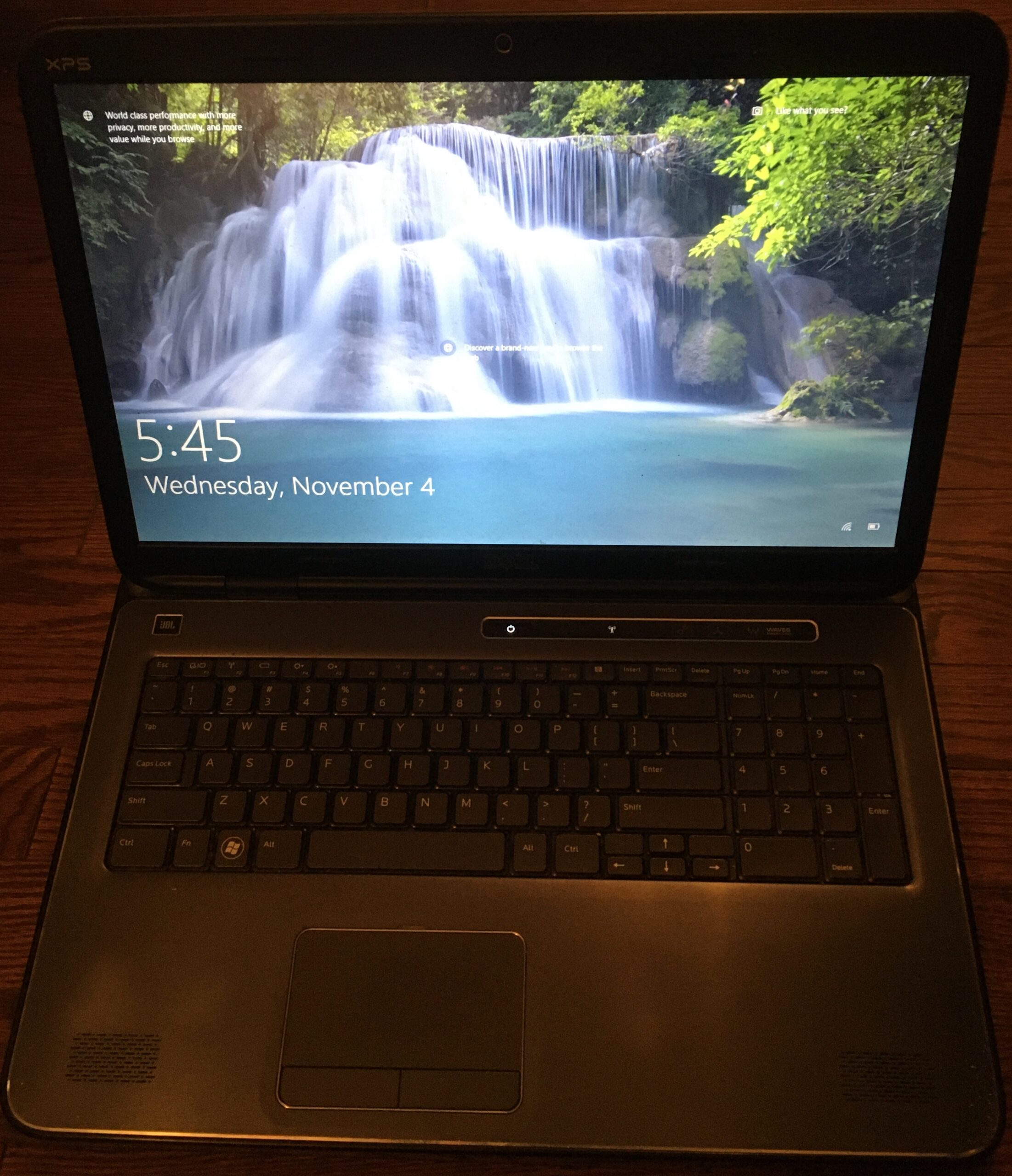
It’s been a long long time, since I bought myself a computer. My old laptop is a DELL XPS, was purchased around 2009:
Since purchasing the XPS lapcrusher, I think that I’ve bought my wife and all the kids a couple machines each, but I’ve always had a work computer that was new enough that I was able to let my personal machine slide.
Old system specs
Specs on the old lapcrusher:
- 19″ screen
- stands over 2″ tall at the back
- Intel Core I3, 64-bit, 4 cores
- 6G Ram
- 500G hard drive, no SSD.
My current work machine is a 4yr old mac (16Mb RAM) and works great, especially since I mainly use it for email and as a dumb terminal to access my Linux NUC consoles using ssh. I have some personal software on the mac that I’d like to uninstall, leaving the work machine for work, and the other for play (Mathematica, LaTex, Julia, …).
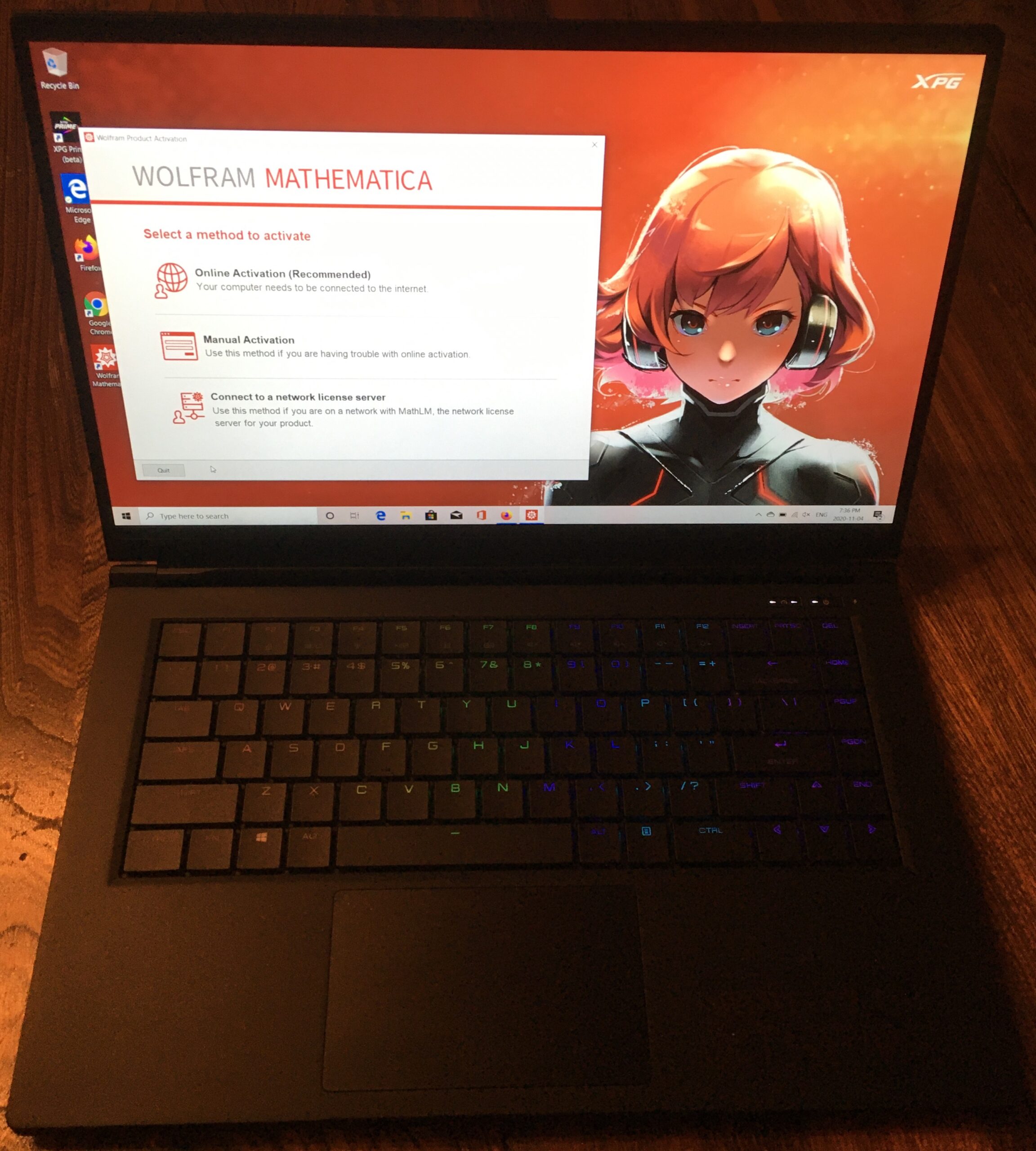
I’ll still install the vpn software for work on the new personal machine so that I can use it as a back up system just in case. Last time I needed a backup system (when the mac was in the shop for battery replacement), I used my wife’s computer. Since Sofia is now mostly working from home (soon to be always working from home), that wouldn’t be an option. Here’s the new system:
New system specs
This splurge is a pretty nicely configured, not top of the line, but it should do nicely for quite a while:
- Display: 15.6″ Full HD IPS | 144HZ | 16:9 | Operating System: Win 10
- Processor: Intel Core i7-9750H Processor (6 core)
- RAM Memory: XPG 32GB 2666MHz DDR4 SO-DIMM (64GB Max)
- Storage: XPG SX8200 1TB NVMe SSD
- Graphics: NVIDIA GeForce GTX 1660Ti 6GB
- USB3.2 Gen 2 x 1 | USB3.2 Gen 2 x 2 | Thunderbolt 3.0 x 1 (REAR)| HDMI x 1 (REAR)
- 4.08lbs
The new machine has a smaller screen size than my old laptop, but the 19″ screen on the old machine was really too big, and with modern screens going so close to the edge, this new one is pretty nice (and has much higher resolution.) If I want a bigger screen, then I’ll hook it up to an external monitor.
On lots of RAM
It doesn’t seem that long ago when I’d just started porting DB2 LUW to 64bit, and most of the “big iron” machines that we got for the testing work barely had more than 4G of ram each. The Solaris kernel guys we worked with at the time told me about the NUMA contortions that they had to use to build machines with large amounts of RAM, because they couldn’t get it close enough together because of heat dissipation issues. Now you can get a personal machine for $1800 CAD with 32G of ram, and 6G of video ram to boot, all tossed into a tiny little form factor! This new machine, not even counting the video ram, has 524288x the memory of my first computer, my old lowly C64 (I’m not counting the little Radio Shack computer that was really my first, as I don’t know how much memory it had — although I am sure it was a whole lot less than 64K.)
C64 Nostalgia.
Incidentally, does anybody else still have their 6402 assembly programming references? I’ve kept mine all these years, moving them around house to house, and taking a peek in them every few years, but I really ought to toss them! I’m sure I couldn’t even give them away.
Remember the zero page addressing of the C64? It was faster to access because it only needed single byte addressing, whereas memory in any other “page” (256 bytes) required two whole bytes to address. That was actually a system where little-endian addressing made a whole lot of sense. If you wanted to change assembler code that did zero page access to “high memory”, then you just added the second byte of additional addressing and could leave your page layout as is.
Windows vs. MacOS
It’s been 4 years since I’ve actively used a Windows machine, and will have to relearn enough to get comfortable with it again (after suffering with the transition to MacOS and finally getting comfortable with it). However, there are some new developments that I’m gung-ho to try, in particular, the new:
- Windows Terminal, and
- The new WSL embedded Linux.
With WSL, I wonder if cygwin is even still a must have? With windows terminal, I’m guessing that putty is a thing of the past (good riddance to cmd, that piece of crap.)