[Click here for a PDF version of this post]
On LinkedIn, James asked for ideas about how to solve What is the total area of ABC? You should be able to solve this! using geometric algebra.
I found a couple ways, and this last variation is pretty cool.
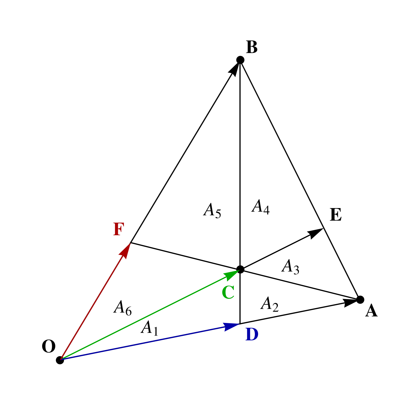
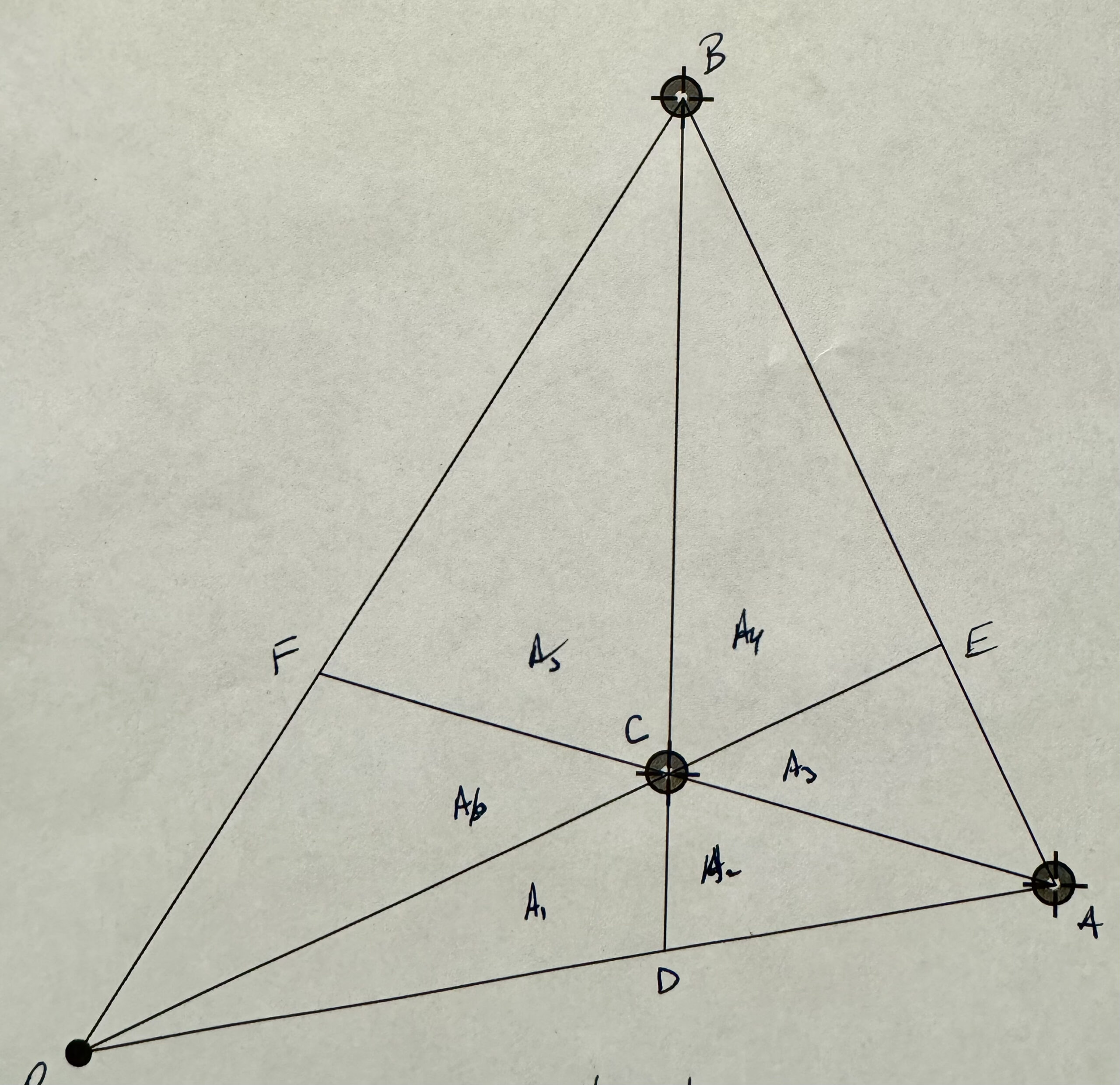
fig. 1. Triangle with given areas.
To start with I’ve re-sketched the triangle with the areas slightly more to scale in fig. 1, where areas \( A_1 = 40, A_2 = 30, A_3 = 35, A_4 = 84 \) are given. The aim is to find the total area \( \sum A_i \).
If we had the vertex and center locations as vectors, we could easily compute the total area, but we don’t. We also don’t know the locations of the edge intersections, but can calculate those, as they satisfy
\begin{equation}\label{eqn:triangle_area_problem:20}
\begin{aligned}
\BD &= s_1 \BA = \BB + t_1 \lr{ \BC – \BB } \\
\BE &= s_2 \BC = \BA + t_2 \lr{ \BB – \BA } \\
\BF &= s_3 \BB = \BA + t_3 \lr{ \BC – \BA }.
\end{aligned}
\end{equation}
It turns out that the problem is over specified, and we will only need \( \BD, \BE \). To find those, we may eliminate the \( t_i \)’s by wedging appropriately (or equivalently, using Cramer’s rule), to find
\begin{equation}\label{eqn:triangle_area_problem:40}
\begin{aligned}
s_1 \BA \wedge \lr{ \BC – \BB } &= \BB \wedge \lr{ \BC – \BB } \\
s_2 \BC \wedge \lr{ \BB – \BA } &= \BA \wedge \lr{ \BB – \BA },
\end{aligned}
\end{equation}
or
\begin{equation}\label{eqn:triangle_area_problem:60}
\begin{aligned}
s_1 &= \frac{\BB \wedge \BC }{\BA \wedge \lr{ \BC – \BB }} \\
s_2 &= \frac{\BA \wedge \BB }{\BC \wedge \lr{ \BB – \BA }}.
\end{aligned}
\end{equation}
Now let’s introduce some scalar area variables, each pseudoscalar multiples of bivector area elements, with \( i = \Be_{1} \Be_2 \)
\begin{equation}\label{eqn:triangle_area_problem:81}
\begin{aligned}
X &= \lr{ \BA \wedge \BB } i^{-1} = \begin{vmatrix} \BA & \BB \end{vmatrix} \\
Y &= \lr{ \BC \wedge \BB } i^{-1} = \begin{vmatrix} \BC & \BB \end{vmatrix} \\
Z &= \lr{ \BA \wedge \BC } i^{-1} = \begin{vmatrix} \BA & \BC \end{vmatrix},
\end{aligned}
\end{equation}
Note that the orientation of all of these has been picked to have a positive orientation matching the figure, and that the
triangle area that we seek for this problem is \( 1/2 \Abs{ \BA \wedge \BB } = X/2 \).
The intersection parameters, after cancelling pseudoscalar factors, are
\begin{equation}\label{eqn:triangle_area_problem:100}
\begin{aligned}
s_1 &= \frac{\BB \wedge \BC }{\BA \wedge \BC – \BA \wedge \BB } = \frac{-Y}{Z – X} \\
s_2 &= \frac{\BA \wedge \BB }{\BC \wedge \BB – \BC \wedge \BA } = \frac{X}{Y + Z},
\end{aligned}
\end{equation}
so the intersection points are
\begin{equation}\label{eqn:triangle_area_problem:120}
\begin{aligned}
\BD &= \BA \frac{Y}{X – Z} \\
\BE &= \BC \frac{X}{Y + Z}.
\end{aligned}
\end{equation}
Observe that both scalar factors are positive (i.e.: \( X > Z \).)
We may now express all the known areas in terms of our area variables
\begin{equation}\label{eqn:triangle_area_problem:140}
\begin{aligned}
A_1 &= \inv{2} \lr{ \BD \wedge \BC } i^{-1} \\
A_1 + A_2 &= \inv{2} \lr{ \BA \wedge \BC } i^{-1} \\
A_1 + A_2 + A_3 &= \inv{2} \lr{ \BA \wedge \BE } i^{-1} \\
A_2 &= \inv{2} \lr{ \lr{\BA – \BD} \wedge \lr{ \BC – \BD } } i^{-1}\\
A_3 &= \inv{2} \lr{ \lr{\BA – \BC} \wedge \lr{ \BE – \BC } } i^{-1}\\
A_5 &= \inv{2} \lr{ \lr{\BB – \BC} \wedge \lr{ \BF – \BC } } i^{-1}.
\end{aligned}
\end{equation}
As mentioned, the problem is over specified, and we can get away with just the first three of these relations to solve for total area. Eliminating \( \BD, \BE \) from those, gives us
\begin{equation}\label{eqn:triangle_area_problem:180}
A_1 = \inv{2} \frac{Y}{X – Z} \lr{ \BA \wedge \BC } i^{-1} = \frac{Z}{2} \lr{ \frac{Y}{X – Z} },
\end{equation}
\begin{equation}\label{eqn:triangle_area_problem:460}
A_1 + A_2 = \inv{2} \lr{ \BA \wedge \BC } i^{-1} = \frac{Z}{2},
\end{equation}
and
\begin{equation}\label{eqn:triangle_area_problem:400}
\begin{aligned}
A_1 + A_2 + A_3 &= \inv{2} \lr{ \BA \wedge \BE } i^{-1} \\
&= \inv{2} \lr{ \BA \wedge \BC } \frac{X}{Y + Z} \\
&= \frac{Z}{2} \frac{X}{Y + Z}.
\end{aligned}
\end{equation}
Let’s eliminate \( Z \) to start with, leaving
\begin{equation}\label{eqn:triangle_area_problem:420}
\begin{aligned}
A_1 \lr{ X – 2 A_1 – 2 A_2 } &= Y \lr{ A_1 + A_2 } \\
\lr{ A_1 + A_2 + A_3 } \lr{ Y + 2 A_1 + 2 A_2 } &= \lr{ A_1 + A_2 } X.
\end{aligned}
\end{equation}
Solving for \( Y \) yields
\begin{equation}\label{eqn:triangle_area_problem:380}
Y = – 2 A_1 – 2 A_2 + \frac{ \lr{A_1 + A_2} X }{ A_1 + A_2 + A_3 } = \lr{ A_1 + A_2 } \lr{ -2 + \frac{X}{A_1 + A_2 + A_3 } },
\end{equation}
and back substution leaves us with a linear equation in \( X \)
\begin{equation}\label{eqn:triangle_area_problem:480}
\lr{ A_1 + A_2}^2 \lr{ -2 + \frac{X}{A_1 + A_2 + A_3 } } = A_1 \lr{ X – 2 A_1 – 2 A_2 }.
\end{equation}
This is easily solved to find
\begin{equation}\label{eqn:triangle_area_problem:500}
\frac{X}{2} = \frac{ \lr{ A_1 + A_2} A_2 \lr{ A_1 + A_2 + A_3 } }{A_2 \lr{ A_1 + A_2} – A_1 A_3 }.
\end{equation}
Plugging in the numeric values for the problem solves it, giving a total triangular area of \( \inv{2} \lr{\BA \wedge \BB } i^{-1} = X/2 = 315 \).
Now, I’ll have to watch the video and see how he solved it.