More on time derivatives of integrals.

June 9, 2024 math and physics play , , , , , , , , , , , , ,

[Click here for a PDF version of this post]

Motivation.

I was asked about geometric algebra equivalents for a couple identities found in [1], one for line integrals
\begin{equation}\label{eqn:more_feynmans_trick:20}
\ddt{} \int_{C(t)} \Bf \cdot d\Bx =
\int_{C(t)} \lr{
\PD{t}{\Bf} + \spacegrad \lr{ \Bv \cdot \Bf } – \Bv \cross \lr{ \spacegrad \cross \Bf }
}
\cdot d\Bx,
\end{equation}
and one for area integrals
\begin{equation}\label{eqn:more_feynmans_trick:40}
\ddt{} \int_{S(t)} \Bf \cdot d\BA =
\int_{S(t)} \lr{
\PD{t}{\Bf} + \Bv \lr{ \spacegrad \cdot \Bf } – \spacegrad \cross \lr{ \Bv \cross \Bf }
}
\cdot d\BA.
\end{equation}

Both of these look questionable at first glance, because neither has boundary term. However, they can be transformed with Stokes theorem to
\begin{equation}\label{eqn:more_feynmans_trick:60}
\ddt{} \int_{C(t)} \Bf \cdot d\Bx
=
\int_{C(t)} \lr{
\PD{t}{\Bf} – \Bv \cross \lr{ \spacegrad \cross \Bf }
}
\cdot d\Bx
+
\evalbar{\Bv \cdot \Bf }{\Delta C},
\end{equation}
and
\begin{equation}\label{eqn:more_feynmans_trick:80}
\ddt{} \int_{S(t)} \Bf \cdot d\BA =
\int_{S(t)} \lr{
\PD{t}{\Bf} + \Bv \lr{ \spacegrad \cdot \Bf }
}
\cdot d\BA

\oint_{\partial S(t)} \lr{ \Bv \cross \Bf } \cdot d\Bx.
\end{equation}
The area integral derivative is now seen to be a variation of one of the special cases of the Leibniz integral rule, see for example [2]. The author admits that the line integral relationship is not well used, and doesn’t show up in the wikipedia page.

My end goal will be to evaluate the derivative of a general multivector line integral
\begin{equation}\label{eqn:more_feynmans_trick:100}
\ddt{} \int_{C(t)} F d\Bx G,
\end{equation}
and area integral
\begin{equation}\label{eqn:more_feynmans_trick:120}
\ddt{} \int_{S(t)} F d^2\Bx G.
\end{equation}
We’ve derived that line integral result in a different fashion previously, but it’s interesting to see a different approach. Perhaps this approach will lend itself nicely to non-scalar integrands?

Prerequisites.

Definition 1.1: Convective derivative.

The convective derivative,
of \( \phi(t, \Bx(t)) \) is defined as
\begin{equation*}
\frac{D \phi}{D t} = \lim_{\Delta t \rightarrow 0} \frac{ \phi(t + \Delta t, \Bx + \Delta t \Bv) – \phi(t, \Bx)}{\Delta t},
\end{equation*}
where \( \Bv = d\Bx/dt \).

Theorem 1.1: Convective derivative.

The convective derivative operator may be written
\begin{equation*}
\frac{D}{D t} = \PD{t}{} + \Bv \cdot \spacegrad.
\end{equation*}

Start proof:

Let’s write
\begin{equation}\label{eqn:more_feynmans_trick:140}
\begin{aligned}
v_0 &= 1 \\
u_0 &= t + v_0 h \\
u_k &= x_k + v_k h, k \in [1,3] \\
\end{aligned}
\end{equation}

The limit, if it exists, must equal the sum of the individual limits
\begin{equation}\label{eqn:more_feynmans_trick:160}
\frac{D \phi}{D t} = \sum_{\alpha = 0}^3 \lim_{\Delta t \rightarrow 0} \frac{ \phi(u_\alpha + v_\alpha h) – \phi(t, Bx)}{h},
\end{equation}
but that is just a sum of derivitives, which can be evaluated by chain rule
\begin{equation}\label{eqn:more_feynmans_trick:180}
\begin{aligned}
\frac{D \phi}{D t}
&= \sum_{\alpha = 0}^{3} \evalbar{ \PD{u_\alpha}{\phi(u_\alpha)} \PD{h}{u_\alpha} }{h = 0} \\
&= \PD{t}{\phi} + \sum_{k = 1}^3 v_k \PD{x_k}{\phi} \\
&= \lr{ \PD{t}{} + \Bv \cdot \spacegrad } \phi.
\end{aligned}
\end{equation}

End proof.

Definition 1.2: Hestenes overdot notation.

We may use a dot or a tick with a derivative operator, to designate the scope of that operator, allowing it to operate bidirectionally, or in a restricted fashion, holding specific multivector elements constant. This is called the Hestenes overdot notation.Illustrating by example, with multivectors \( F, G \), and allowing the gradient to act bidirectionally, we have
\begin{equation*}
\begin{aligned}
F \spacegrad G
&=
\dot{F} \dot{\spacegrad} G
+
F \dot{\spacegrad} \dot{G} \\
&=
\sum_i \lr{ \partial_i F } \Be_i G + \sum_i F \Be_i \lr{ \partial_i G }.
\end{aligned}
\end{equation*}
The last step is a precise statement of the meaning of the overdot notation, showing that we hold the position of the vector elements of the gradient constant, while the (scalar) partials are allowed to commute, acting on the designated elements.

We will need one additional identity

Lemma 1.1: Gradient of dot product (one constant vector.)

Given vectors \( \Ba, \Bb \) the gradient of their dot product is given by
\begin{equation*}
\spacegrad \lr{ \Ba \cdot \Bb }
= \lr{ \Bb \cdot \spacegrad } \Ba – \Bb \cdot \lr{ \spacegrad \wedge \Ba }
+ \lr{ \Ba \cdot \spacegrad } \Bb – \Ba \cdot \lr{ \spacegrad \wedge \Bb }.
\end{equation*}
If \( \Bb \) is constant, this reduces to
\begin{equation*}
\spacegrad \lr{ \Ba \cdot \Bb }
=
\dot{\spacegrad} \lr{ \dot{\Ba} \cdot \Bb }
= \lr{ \Bb \cdot \spacegrad } \Ba – \Bb \cdot \lr{ \spacegrad \wedge \Ba }.
\end{equation*}

Start proof:

The \( \Bb \) constant case is trivial to prove. We use \( \Ba \cdot \lr{ \Bb \wedge \Bc } = \lr{ \Ba \cdot \Bb} \Bc – \Bb \lr{ \Ba \cdot \Bc } \), and simply expand the vector, curl dot product
\begin{equation}\label{eqn:more_feynmans_trick:200}
\Bb \cdot \lr{ \spacegrad \wedge \Ba }
=
\Bb \cdot \lr{ \dot{\spacegrad} \wedge \dot{\Ba} }
= \lr{ \Bb \cdot \dot{\spacegrad} } \dot{\Ba} – \dot{\spacegrad} \lr{ \dot{\Ba} \cdot \Bb }. \end{equation}
Rearrangement proves that \( \Bb \) constant identity. The more general statement follows from a chain rule evaluation of the gradient, holding each vector constant in turn
\begin{equation}\label{eqn:more_feynmans_trick:320}
\spacegrad \lr{ \Ba \cdot \Bb }
=
\dot{\spacegrad} \lr{ \dot{\Ba} \cdot \Bb }
+
\dot{\spacegrad} \lr{ \dot{\Bb} \cdot \Ba }.
\end{equation}

End proof.

Time derivative of a line integral of a vector field.

We now have all our tools assembled, and can proceed to evaluate the derivative of the line integral. We want to show that

Theorem 1.2:

Given a path parameterized by \( \Bx(\lambda) \), where \( d\Bx = (\PDi{\lambda}{\Bx}) d\lambda \), with points along a \( C(t) \) moving through space at a velocity \( \Bv(\Bx(\lambda)) \), and a vector function \( \Bf = \Bf(t, \Bx(\lambda)) \),
\begin{equation*}
\ddt{} \int_{C(t)} \Bf \cdot d\Bx =
\int_{C(t)} \lr{
\PD{t}{\Bf} + \spacegrad \lr{ \Bf \cdot \Bv } + \Bv \cdot \lr{ \spacegrad \wedge \Bf}
} \cdot d\Bx
\end{equation*}

Start proof:

I’m going to avoid thinking about the rigorous details, like any requirements for curve continuity and smoothness. We will however, specify that the end points are given by \( [\lambda_1, \lambda_2] \). Expanding out the parameterization, we seek to evaluate
\begin{equation}\label{eqn:more_feynmans_trick:240}
\int_{C(t)} \Bf \cdot d\Bx
=
\int_{\lambda_1}^{\lambda_2} \Bf(t, \Bx(\lambda) ) \cdot \frac{\partial \Bx}{\partial \lambda} d\lambda.
\end{equation}
The parametric form nicely moves all the boundary time dependence into the integrand, allowing us to write
\begin{equation}\label{eqn:more_feynmans_trick:260}
\begin{aligned}
\ddt{} \int_{C(t)} \Bf \cdot d\Bx
&=
\lim_{\Delta t \rightarrow 0}
\inv{\Delta t}
\int_{\lambda_1}^{\lambda_2}
\lr{ \Bf(t + \Delta t, \Bx(\lambda) + \Delta t \Bv(\Bx(\lambda) ) \cdot \frac{\partial}{\partial \lambda} \lr{ \Bx + \Delta t \Bv(\Bx(\lambda)) } – \Bf(t, \Bx(\lambda)) \cdot \frac{\partial \Bx}{\partial \lambda} } d\lambda \\
&=
\lim_{\Delta t \rightarrow 0}
\inv{\Delta t}
\int_{\lambda_1}^{\lambda_2}
\lr{ \Bf(t + \Delta t, \Bx(\lambda) + \Delta t \Bv(\Bx(\lambda) ) – \Bf(t, \Bx)} \cdot \frac{\partial \Bx}{\partial \lambda} d\lambda \\
&\quad+
\lim_{\Delta t \rightarrow 0}
\int_{\lambda_1}^{\lambda_2}
\Bf(t + \Delta t, \Bx(\lambda) + \Delta t \Bv(\Bx(\lambda) )) \cdot \PD{\lambda}{}\Bv(\Bx(\lambda)) d\lambda \\
&=
\int_{\lambda_1}^{\lambda_2}
\frac{D \Bf}{Dt} \cdot \frac{\partial \Bx}{\partial \lambda} d\lambda +
\lim_{\Delta t \rightarrow 0}
\int_{\lambda_1}^{\lambda_2}
\Bf(t + \Delta t, \Bx(\lambda) + \Delta t \Bv(\Bx(\lambda) \cdot \frac{\partial}{\partial \lambda} \Bv(\Bx(\lambda)) d\lambda \\
&=
\int_{\lambda_1}^{\lambda_2}
\lr{ \PD{t}{\Bf} + \lr{ \Bv \cdot \spacegrad } \Bf } \cdot \frac{\partial \Bx}{\partial \lambda} d\lambda
+
\int_{\lambda_1}^{\lambda_2}
\Bf \cdot \frac{\partial \Bv}{\partial \lambda} d\lambda
\end{aligned}
\end{equation}
At this point, we have a \( d\Bx \) in the first integrand, and a \( d\Bv \) in the second. We can expand the second integrand, evaluating the derivative using chain rule to find
\begin{equation}\label{eqn:more_feynmans_trick:280}
\begin{aligned}
\Bf \cdot \PD{\lambda}{\Bv}
&=
\sum_i \Bf \cdot \PD{x_i}{\Bv} \PD{\lambda}{x_i} \\
&=
\sum_{i,j} f_j \PD{x_i}{v_j} \PD{\lambda}{x_i} \\
&=
\sum_{j} f_j \lr{ \spacegrad v_j } \cdot \PD{\lambda}{\Bx} \\
&=
\sum_{j} \lr{ \dot{\spacegrad} f_j \dot{v_j} } \cdot \PD{\lambda}{\Bx} \\
&=
\dot{\spacegrad} \lr{ \Bf \cdot \dot{\Bv} } \cdot \PD{\lambda}{\Bx}.
\end{aligned}
\end{equation}
Substitution gives
\begin{equation}\label{eqn:more_feynmans_trick:300}
\begin{aligned}
\ddt{} \int_{C(t)} \Bf \cdot d\Bx
&=
\int_{C(t)}
\lr{ \PD{t}{\Bf} + \lr{ \Bv \cdot \spacegrad } \Bf + \dot{\spacegrad} \lr{ \Bf \cdot \dot{\Bv} } } \cdot \frac{\partial \Bx}{\partial \lambda} d\lambda \\
&=
\int_{C(t)}
\lr{ \PD{t}{\Bf}
+ \spacegrad \lr{ \Bf \cdot \Bv }
+ \lr{ \Bv \cdot \spacegrad } \Bf
– \dot{\spacegrad} \lr{ \dot{\Bf} \cdot \Bv }
} \cdot d\Bx \\
&=
\int_{C(t)}
\lr{ \PD{t}{\Bf}
+ \spacegrad \lr{ \Bf \cdot \Bv }
+ \Bv \cdot \lr{ \spacegrad \wedge \Bf }
} \cdot d\Bx,
\end{aligned}
\end{equation}
where the last simplification utilizes lemma 1.1.

End proof.

Since \( \Ba \cdot \lr{ \Bb \wedge \Bc } = -\Ba \cross \lr{ \Bb \cross \Bc } \), observe that we have also recovered \ref{eqn:more_feynmans_trick:20}.

Time derivative of a line integral of a bivector field.

For a bivector line integral, we have

Theorem 1.3:

Given a path parameterized by \( \Bx(\lambda) \), where \( d\Bx = (\PDi{\lambda}{\Bx}) d\lambda \), with points along a \( C(t) \) moving through space at a velocity \( \Bv(\Bx(\lambda)) \), and a bivector function \( B = B(t, \Bx(\lambda)) \),
\begin{equation*}
\ddt{} \int_{C(t)} B \cdot d\Bx =
\int_{C(t)}
\PD{t}{B} \cdot d\Bx + \lr{ d\Bx \cdot \spacegrad } \lr{ B \cdot \Bv } + \lr{ \lr{ \Bv \wedge d\Bx } \cdot \spacegrad } \cdot B.
\end{equation*}

Start proof:

Skipping the steps that follow our previous proceedure exactly, we have
\begin{equation}\label{eqn:more_feynmans_trick:340}
\ddt{} \int_{C(t)} B \cdot d\Bx =
\int_{C(t)}
\PD{t}{B} \cdot d\Bx + \lr{ \Bv \cdot \spacegrad } B \cdot d\Bx + B \cdot d\Bv.
\end{equation}
Since
\begin{equation}\label{eqn:more_feynmans_trick:360}
\begin{aligned}
B \cdot d\Bv
&= B \cdot \PD{\lambda}{\Bv} d\lambda \\
&= B \cdot \PD{x_i}{\Bv} \PD{\lambda}{x_i} d\lambda \\
&= B \cdot \lr{ \lr{ d\Bx \cdot \spacegrad } \Bv },
\end{aligned}
\end{equation}
we have
\begin{equation}\label{eqn:more_feynmans_trick:380}
\ddt{} \int_{C(t)} B \cdot d\Bx
=
\int_{C(t)}
\PD{t}{B} \cdot d\Bx + \lr{ \Bv \cdot \spacegrad } B \cdot d\Bx + B \cdot \lr{ \lr{ d\Bx \cdot \spacegrad } \Bv } \\
\end{equation}
Let’s reduce the two last terms in this integrand
\begin{equation}\label{eqn:more_feynmans_trick:400}
\begin{aligned}
\lr{ \Bv \cdot \spacegrad } B \cdot d\Bx + B \cdot \lr{ \lr{ d\Bx \cdot \spacegrad } \Bv }
&=
\lr{ \Bv \cdot \spacegrad } B \cdot d\Bx –
\lr{ d\Bx \cdot \dot{\spacegrad} } \lr{ \dot{\Bv} \cdot B } \\
&=
\lr{ \Bv \cdot \spacegrad } B \cdot d\Bx
– \lr{ d\Bx \cdot \spacegrad} \lr{ \Bv \cdot B }
+ \lr{ d\Bx \cdot \dot{\spacegrad} } \lr{ \Bv \cdot \dot{B} } \\
&=
\lr{ d\Bx \cdot \spacegrad} \lr{ B \cdot \Bv }
+ \lr{ \Bv \cdot \dot{\spacegrad} } \dot{B} \cdot d\Bx
+ \lr{ d\Bx \cdot \dot{\spacegrad} } \lr{ \Bv \cdot \dot{B} } \\
&=
\lr{ d\Bx \cdot \spacegrad} \lr{ B \cdot \Bv }
+ \lr{ \Bv \lr{ d\Bx \cdot \spacegrad } – d\Bx \lr{ \Bv \cdot \spacegrad } } \cdot B \\
&=
\lr{ d\Bx \cdot \spacegrad} \lr{ B \cdot \Bv }
+ \lr{ \lr{ \Bv \wedge d\Bx } \cdot \spacegrad } \cdot B.
\end{aligned}
\end{equation}
Back substitution finishes the job.

End proof.

Time derivative of a multivector line integral.

Theorem 1.4: Time derivative of multivector line integral.

Given a path parameterized by \( \Bx(\lambda) \), where \( d\Bx = (\PDi{\lambda}{\Bx}) d\lambda \), with points along a \( C(t) \) moving through space at a velocity \( \Bv(\Bx(\lambda)) \), and multivector functions \( M = M(t, \Bx(\lambda)), N = N(t, \Bx(\lambda)) \),
\begin{equation*}
\ddt{} \int_{C(t)} M d\Bx N =
\int_{C(t)}
\frac{D}{D t} M d\Bx N + M \lr{ \lr{ d\Bx \cdot \dot{\spacegrad} } \dot{\Bv} } N.
\end{equation*}

It is useful to write this out explicitly for clarity
\begin{equation}\label{eqn:more_feynmans_trick:420}
\ddt{} \int_{C(t)} M d\Bx N =
\int_{C(t)}
\PD{t}{M} d\Bx N + M d\Bx \PD{t}{N}
+ \dot{M} \lr{ \Bv \cdot \dot{\spacegrad} } N
+ M \lr{ \Bv \cdot \dot{\spacegrad} } \dot{N}
+ M \lr{ \lr{ d\Bx \cdot \dot{\spacegrad} } \dot{\Bv} } N.
\end{equation}

Proof is left to the reader, but follows the patterns above.

It’s not obvious whether there is a nice way to reduce this, as we did for the scalar valued line integral of a vector function, and the vector valued line integral of a bivector function. In particular, our vector and bivector results had \( \spacegrad \lr{ \Bf \cdot \Bv } \), and \( \spacegrad \lr{ B \cdot \Bv } \) terms respectively, which allows for the boundary term to be evaluated using Stokes’ theorem. Is such a manipulation possible here?

Coming later: surface integrals!

References

[1] Nicholas Kemmer. Vector Analysis: A physicist’s guide to the mathematics of fields in three dimensions. CUP Archive, 1977.

[2] Wikipedia contributors. Leibniz integral rule — Wikipedia, the free encyclopedia. https://en.wikipedia.org/w/index.php?title=Leibniz_integral_rule&oldid=1223666713, 2024. [Online; accessed 22-May-2024].

Multivector form of Leibniz integral theorem for line integrals.

June 2, 2024 math and physics play , , , , ,

[Click here for a PDF version of this post]

Goal.

Here we will explore the multivector form of the Leibniz integral theorem (aka. Feynman’s trick in one dimension), as discussed in [1].

Given a boundary \( \Omega(t) \) that varies in time, we seek to evaluate
\begin{equation}\label{eqn:LeibnizIntegralTheorem:20}
\ddt{} \int_{\Omega(t)} F d^p \Bx \lrpartial G.
\end{equation}
Recall that when the bounding volume is fixed, we have
\begin{equation}\label{eqn:LeibnizIntegralTheorem:40}
\int_{\Omega} F d^p \Bx \lrpartial G = \int_{\partial \Omega} F d^{p-1} \Bx G,
\end{equation}
and expect a few terms that are variations of the RHS if we take derivatives.

Simplest case: scalar function, one variable.

With
\begin{equation}\label{eqn:LeibnizIntegralTheorem:60}
A(t) = \int_{a(t)}^{b(t)} f(u, t) du,
\end{equation}
If we can find an antiderivative, such that
\begin{equation}\label{eqn:LeibnizIntegralTheorem:80}
\PD{u}{F(u,t)} = f(u, t),
\end{equation}
or
\begin{equation}\label{eqn:LeibnizIntegralTheorem:90}
F(u, t) = \int f(u, t) du.
\end{equation}
The integral is made trivial
\begin{equation}\label{eqn:LeibnizIntegralTheorem:100}
\begin{aligned}
A(t)
&=
\int_{a(t)}^{b(t)} f(u, t) du \\
&=
\int_{a(t)}^{b(t)} \PD{u}{F(u,t)} du \\
&= F( b(t), t ) – F( a(t), t ).
\end{aligned}
\end{equation}
Should we attempt to take derivatives, we have a contribution from the first parameter that is entirely dependent on the boundary, and a contribution from the second parameter that is entirely independent of the boundary. That is
\begin{equation}\label{eqn:LeibnizIntegralTheorem:120}
\begin{aligned}
\ddt{} \int_{a(t)}^{b(t)} f(u, t) du
&=
\PD{b}{ F } \PD{t}{b}
-\PD{a}{ F } \PD{t}{a}
+ \evalrange{\PD{t}{F(u, t)}}{u = a(t)}{b(t)} \\
&=
f(b(t), t) b'(t) –
f(a(t), t) a'(t)
+ \int_{a(t)}^{b(t)} \PD{t}{} f(u, t) du.
\end{aligned}
\end{equation}
In the second step, the antiderivative function \( F \) has been restated in it’s original integral form \ref{eqn:LeibnizIntegralTheorem:90}. We are able to take the derivative into the integral, since we first evaluate that derivative, independent of the boundary, and then evaluate the result at the respective end points of the boundary.

Next simplest case: Multivector line integral (perfect derivative.)

Given an \( N \) dimensional vector space, and a path parameterized by vector \( \Bx = \Bx(u) \). The line integral special case of the fundamental theorem of calculus is found by evaluating
\begin{equation}\label{eqn:LeibnizIntegralTheorem:140}
\int F(u) d\Bx \lrpartial G(u),
\end{equation}
where \( F, G \) are multivectors, and
\begin{equation}\label{eqn:LeibnizIntegralTheorem:160}
\begin{aligned}
d\Bx &= \PD{u}{\Bx} du = \Bx_u du \\
\lrpartial &= \Bx^u \stackrel{ \leftrightarrow }{\PD{u}{}},
\end{aligned}
\end{equation}
where \( \Bx_u \Bx^u = \Bx_u \cdot \Bx^u = 1 \).

Evaluating the integral, we have
\begin{equation}\label{eqn:LeibnizIntegralTheorem:180}
\begin{aligned}
\int F(u) d\Bx \lrpartial G(u)
&=
\int F(u) \Bx_u du \Bx^u \stackrel{ \leftrightarrow }{\PD{u}{}} G(u) \\
&=
\int du \PD{u}{} \lr{ F(u) G(u) } \\
&=
F(u) G(u).
\end{aligned}
\end{equation}

If we allow \( F, G, \Bx \) to each have time dependence
\begin{equation}\label{eqn:LeibnizIntegralTheorem:200}
\begin{aligned}
F &= F(u, t) \\
G &= G(u, t) \\
\Bx &= \Bx(u, t),
\end{aligned}
\end{equation}
so we have
\begin{equation}\label{eqn:LeibnizIntegralTheorem:220}
\ddt{} \int_{u = a(t)}^{b(t)} F(u, t) d\Bx \lrpartial G(u, t)
=
\evalrange{ \ddt{u} \PD{u}{} \lr{ F(u, t) G(u, t) } }{u = a(t)}{b(t)}
+ \evalrange{\ddt{} \lr{ F(u, t) G(u, t) } }{u = a(t)}{b(t)}
.
\end{equation}

General multivector line integral.

Now suppose that we have a general multivector line integral
\begin{equation}\label{eqn:LeibnizIntegralTheorem:240}
A(t) = \int_{a(t)}^{b(t)} F(u, t) d\Bx G(u, t),
\end{equation}
where \( d\Bx = \Bx_u du \), \( \Bx_u = \partial \Bx(u, t)/\partial u \). Writing out the integrand explicitly, we have
\begin{equation}\label{eqn:LeibnizIntegralTheorem:260}
A(t) = \int_{a(t)}^{b(t)} du F(u, t) \Bx_u(u, t) G(u, t).
\end{equation}
Following our logic with the first scalar case, let
\begin{equation}\label{eqn:LeibnizIntegralTheorem:280}
\PD{u}{B(u, t)} = F(u, t) \Bx_u(u, t) G(u, t).
\end{equation}
We can now evaluate the derivative
\begin{equation}\label{eqn:LeibnizIntegralTheorem:300}
\ddt{A(t)} = \evalrange{ \ddt{u} \PD{u}{B} }{u = a(t)}{b(t)} + \evalrange{ \PD{t}{}B(u, t) }{u = a(t)}{b(t)}.
\end{equation}
Writing \ref{eqn:LeibnizIntegralTheorem:280} in integral form, we have
\begin{equation}\label{eqn:LeibnizIntegralTheorem:320}
B(u, t) = \int du F(u, t) \Bx_u(u, t) G(u, t),
\end{equation}
so
\begin{equation}\label{eqn:LeibnizIntegralTheorem:340}
\begin{aligned}
\ddt{A(t)}
&= \evalrange{ \ddt{u} \PD{u}{B} }{u = a(t)}{b(t)} +
\evalbar{ \PD{t’}{} \int_{a(t)}^{b(t)} du F(u, t’) d\Bx_u(u, t’) G(u, t’) }{t’ = t} \\
&= \evalrange{ \ddt{u} F(u, t) \Bx_u(u, t) G(u, t) }{u = a(t)}{b(t)} +
\int_{a(t)}^{b(t)} \PD{t}{} F(u, t) d\Bx(u, t) G(u, t),
\end{aligned}
\end{equation}
so
\begin{equation}\label{eqn:LeibnizIntegralTheorem:360}
\ddt{} \int_{a(t)}^{b(t)} F(u, t) d\Bx(u, t) G(u, t)
= \evalrange{ F(u, t) \ddt{\Bx}(u, t) G(u, t) }{u = a(t)}{b(t)} +
\int_{a(t)}^{b(t)} \PD{t}{} F(u, t) d\Bx(u, t) G(u, t).
\end{equation}

This is perhaps clearer, if just written as:
\begin{equation}\label{eqn:LeibnizIntegralTheorem:380}
\ddt{} \int_{a(t)}^{b(t)} F d\Bx G
= \evalrange{ F \ddt{\Bx} G }{u = a(t)}{b(t)} +
\int_{a(t)}^{b(t)} \PD{t}{} F d\Bx G.
\end{equation}
As a check, it’s worth pointing out that we can recover the one dimensional result, writing \( \Bx = u \Be_1 \), \( f = F \Be_1^{-1} \), and \( G = 1 \), for
\begin{equation}\label{eqn:LeibnizIntegralTheorem:400}
\ddt{} \int_{a(t)}^{b(t)} f du
= \evalrange{ f(u) \ddt{u} }{u = a(t)}{b(t)} +
\int_{a(t)}^{b(t)} du \PD{t}{f}.
\end{equation}

Next steps.

I’ve tried a couple times on paper to do surface integral variations of this (allowing the surface to vary with time), and don’t think that I’ve gotten it right. Will try again (or perhaps just look it up and see what the result is supposed to look like, then see how that translates into the GC formalism.)

References

[1] Wikipedia contributors. Leibniz integral rule — Wikipedia, the free encyclopedia. https://en.wikipedia.org/w/index.php?title=Leibniz_integral_rule&oldid=1223666713, 2024. [Online; accessed 22-May-2024].

A walnut sheath project for a kitchen knife.

May 29, 2024 Wood working , , , , , , , , , , ,

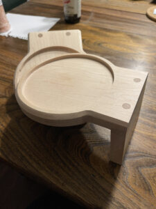
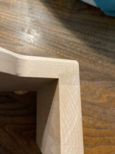
My daughter Aurora has a (beautiful and wonderfully sharp) kitchen knife that has a lost sheath, so I made a replacement sheath from a 1″ thick piece of walnut that had really nice figure.  Here is the final result

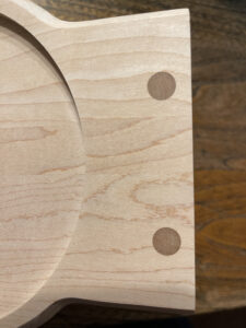
The sheath has two halves, with a routered out section in the interior that the knife blade fits into.  As this was a one time project, I didn’t make a template for that interior routering, but just did it by hand.  The inside doesn’t look great, but that part doesn’t really show.  Four little 5mm magnets in each piece allow the two halves to snap together around the blade.

I posted a video showing the knife on Google’s censorshipTube, and got one critical comment about (paraphrasing) that was along the lines of “just one twist of the blade with pop the halves, voiding any safety that the sheath provides.”  That comment is true enough, but it is not as if this sheath is going to be used on a knife belt.  Instead this is for static situations, where the knife isn’t in use, and for storage.  It’s also for just plain looking awesome, while the blade is not in use, which I think it does.  The magnet latching has just enough strength that it stays on when desired, and comes off when desired.


On the construction.

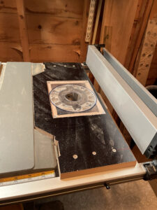
The board I started with was a strange shaped one with a large defect, and a U shape.  I cut off a 5″ strip (one arm of the U), and further cut that down the center into two 3/8″ halves.  I don’t have a band saw, so I scored it down the center on the table saw with a very thin kerf blade (actually a thin 7″ skill saw blade), and then used a hand saw to finish the resawing process.  Some hand planing after that left me with two flattish pieces.

Cutting the board down the center released a lot of pressure, letting the two pieces bow considerably.  In fact, I was quite surprised just how much bowing occurred after that sawing.

I dealt wit the bowing by flattening the two halves to a thinner width than I had originally intended.  I did the flattening with my planer (I don’t have a jointer), shimming the pieces and hot gluing them down to a flattening jig (i.e.: a board), then running them through the planer until I had two flat’ish boards, instead of my two bowed pieces.  I started at close to 1″ thick, and ended up with a total thickness of about 1/2″ instead!

Once I had two flat pieces, it was just a matter of shaping them, cutting a cavity for the blade, embedding the magnets, some sanding, oiling and finally waxing.

Embedding the magnets was actually a bit tricky.  I ended up buying a set of metric brad point drill bits to get the correct sized hole (and had to be very careful to not go too deep as the brad point bits have a long tip.)  I used a bit of epoxy glue to set the magnets, but the hole clearance was so tight that too much epoxy didn’t let the magnet go all the way in (i.e.: too tight for squeeze out.)

Triangle area problem: REVISITED.

March 31, 2024 math and physics play , , , , ,

[Click here for a PDF version of this post]

On LinkedIn, James asked for ideas about how to solve What is the total area of ABC? You should be able to solve this! using geometric algebra.

I found a couple ways, and this last variation is pretty cool.

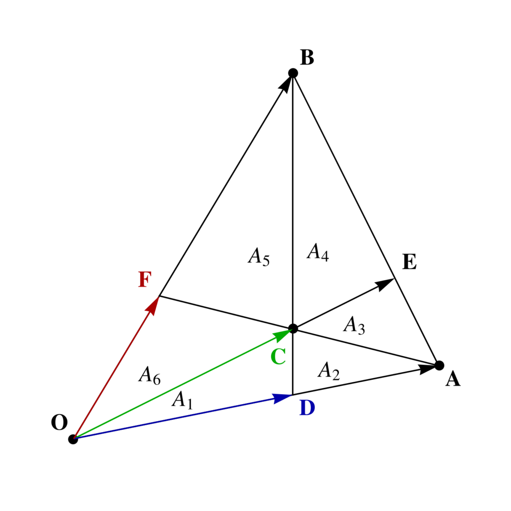
fig. 1. Triangle with given areas.

To start with I’ve re-sketched the triangle with the areas slightly more to scale in fig. 1, where areas \( A_1 = 40, A_2 = 30, A_3 = 35, A_4 = 84 \) are given. The aim is to find the total area \( \sum A_i \).

If we had the vertex and center locations as vectors, we could easily compute the total area, but we don’t. We also don’t know the locations of the edge intersections, but can calculate those, as they satisfy
\begin{equation}\label{eqn:triangle_area_problem:20}
\begin{aligned}
\BD &= s_1 \BA = \BB + t_1 \lr{ \BC – \BB } \\
\BE &= s_2 \BC = \BA + t_2 \lr{ \BB – \BA } \\
\BF &= s_3 \BB = \BA + t_3 \lr{ \BC – \BA }.
\end{aligned}
\end{equation}
It turns out that the problem is over specified, and we will only need \( \BD, \BE \). To find those, we may eliminate the \( t_i \)’s by wedging appropriately (or equivalently, using Cramer’s rule), to find
\begin{equation}\label{eqn:triangle_area_problem:40}
\begin{aligned}
s_1 \BA \wedge \lr{ \BC – \BB } &= \BB \wedge \lr{ \BC – \BB } \\
s_2 \BC \wedge \lr{ \BB – \BA } &= \BA \wedge \lr{ \BB – \BA },
\end{aligned}
\end{equation}
or
\begin{equation}\label{eqn:triangle_area_problem:60}
\begin{aligned}
s_1 &= \frac{\BB \wedge \BC }{\BA \wedge \lr{ \BC – \BB }} \\
s_2 &= \frac{\BA \wedge \BB }{\BC \wedge \lr{ \BB – \BA }}.
\end{aligned}
\end{equation}
Now let’s introduce some scalar area variables, each pseudoscalar multiples of bivector area elements, with \( i = \Be_{1} \Be_2 \)
\begin{equation}\label{eqn:triangle_area_problem:81}
\begin{aligned}
X &= \lr{ \BA \wedge \BB } i^{-1} = \begin{vmatrix} \BA & \BB \end{vmatrix} \\
Y &= \lr{ \BC \wedge \BB } i^{-1} = \begin{vmatrix} \BC & \BB \end{vmatrix} \\
Z &= \lr{ \BA \wedge \BC } i^{-1} = \begin{vmatrix} \BA & \BC \end{vmatrix},
\end{aligned}
\end{equation}
Note that the orientation of all of these has been picked to have a positive orientation matching the figure, and that the
triangle area that we seek for this problem is \( 1/2 \Abs{ \BA \wedge \BB } = X/2 \).

The intersection parameters, after cancelling pseudoscalar factors, are
\begin{equation}\label{eqn:triangle_area_problem:100}
\begin{aligned}
s_1 &= \frac{\BB \wedge \BC }{\BA \wedge \BC – \BA \wedge \BB } = \frac{-Y}{Z – X} \\
s_2 &= \frac{\BA \wedge \BB }{\BC \wedge \BB – \BC \wedge \BA } = \frac{X}{Y + Z},
\end{aligned}
\end{equation}
so the intersection points are
\begin{equation}\label{eqn:triangle_area_problem:120}
\begin{aligned}
\BD &= \BA \frac{Y}{X – Z} \\
\BE &= \BC \frac{X}{Y + Z}.
\end{aligned}
\end{equation}
Observe that both scalar factors are positive (i.e.: \( X > Z \).)

We may now express all the known areas in terms of our area variables
\begin{equation}\label{eqn:triangle_area_problem:140}
\begin{aligned}
A_1 &= \inv{2} \lr{ \BD \wedge \BC } i^{-1} \\
A_1 + A_2 &= \inv{2} \lr{ \BA \wedge \BC } i^{-1} \\
A_1 + A_2 + A_3 &= \inv{2} \lr{ \BA \wedge \BE } i^{-1} \\
A_2 &= \inv{2} \lr{ \lr{\BA – \BD} \wedge \lr{ \BC – \BD } } i^{-1}\\
A_3 &= \inv{2} \lr{ \lr{\BA – \BC} \wedge \lr{ \BE – \BC } } i^{-1}\\
A_5 &= \inv{2} \lr{ \lr{\BB – \BC} \wedge \lr{ \BF – \BC } } i^{-1}.
\end{aligned}
\end{equation}

As mentioned, the problem is over specified, and we can get away with just the first three of these relations to solve for total area. Eliminating \( \BD, \BE \) from those, gives us
\begin{equation}\label{eqn:triangle_area_problem:180}
A_1 = \inv{2} \frac{Y}{X – Z} \lr{ \BA \wedge \BC } i^{-1} = \frac{Z}{2} \lr{ \frac{Y}{X – Z} },
\end{equation}
\begin{equation}\label{eqn:triangle_area_problem:460}
A_1 + A_2 = \inv{2} \lr{ \BA \wedge \BC } i^{-1} = \frac{Z}{2},
\end{equation}
and
\begin{equation}\label{eqn:triangle_area_problem:400}
\begin{aligned}
A_1 + A_2 + A_3 &= \inv{2} \lr{ \BA \wedge \BE } i^{-1} \\
&= \inv{2} \lr{ \BA \wedge \BC } \frac{X}{Y + Z} \\
&= \frac{Z}{2} \frac{X}{Y + Z}.
\end{aligned}
\end{equation}

Let’s eliminate \( Z \) to start with, leaving
\begin{equation}\label{eqn:triangle_area_problem:420}
\begin{aligned}
A_1 \lr{ X – 2 A_1 – 2 A_2 } &= Y \lr{ A_1 + A_2 } \\
\lr{ A_1 + A_2 + A_3 } \lr{ Y + 2 A_1 + 2 A_2 } &= \lr{ A_1 + A_2 } X.
\end{aligned}
\end{equation}
Solving for \( Y \) yields
\begin{equation}\label{eqn:triangle_area_problem:380}
Y = – 2 A_1 – 2 A_2 + \frac{ \lr{A_1 + A_2} X }{ A_1 + A_2 + A_3 } = \lr{ A_1 + A_2 } \lr{ -2 + \frac{X}{A_1 + A_2 + A_3 } },
\end{equation}
and back substution leaves us with a linear equation in \( X \)
\begin{equation}\label{eqn:triangle_area_problem:480}
\lr{ A_1 + A_2}^2 \lr{ -2 + \frac{X}{A_1 + A_2 + A_3 } } = A_1 \lr{ X – 2 A_1 – 2 A_2 }.
\end{equation}

This is easily solved to find
\begin{equation}\label{eqn:triangle_area_problem:500}
\frac{X}{2} = \frac{ \lr{ A_1 + A_2} A_2 \lr{ A_1 + A_2 + A_3 } }{A_2 \lr{ A_1 + A_2} – A_1 A_3 }.
\end{equation}
Plugging in the numeric values for the problem solves it, giving a total triangular area of \( \inv{2} \lr{\BA \wedge \BB } i^{-1} = X/2 = 315 \).

Now, I’ll have to watch the video and see how he solved it.

Triangle area problem

March 30, 2024 math and physics play , , , , , ,

[Click here for a PDF version of this post]

On LinkedIn, James asked for ideas about how to solve What is the total area of ABC? You should be able to solve this! using geometric algebra.

I found one way, but suspect it’s not the easiest way to solve the problem.

To start with I’ve re-sketched the triangle with the areas slightly more to scale in fig. 1, where areas \( A_1, A_2, A_3, A_5\) are given. The aim is to find the total area \( \sum A_i \).

fig. 1. Triangle with given areas.


If we had the vertex and center locations as vectors, we could easily compute the total area, but we don’t. We also don’t know the locations of the edge intersections, but can calculate those, as they satisfy
\begin{equation}\label{eqn:triangle_area_problem:20}
\begin{aligned}
\BD &= s_1 \BA = \BB + t_1 \lr{ \BC – \BB } \\
\BE &= s_2 \BC = \BA + t_2 \lr{ \BB – \BA } \\
\BF &= s_3 \BB = \BA + t_3 \lr{ \BC – \BA }.
\end{aligned}
\end{equation}
Eliminating the \( t_i \) constants by wedging appropriately (or equivalently, using Cramer’s rule), we find
\begin{equation}\label{eqn:triangle_area_problem:40}
\begin{aligned}
s_1 \BA \wedge \lr{ \BC – \BB } &= \BB \wedge \lr{ \BC – \BB } \\
s_2 \BC \wedge \lr{ \BB – \BA } &= \BA \wedge \lr{ \BB – \BA } \\
s_3 \BB \wedge \lr{ \BC – \BA } &= \BA \wedge \lr{ \BC – \BA },
\end{aligned}
\end{equation}
or
\begin{equation}\label{eqn:triangle_area_problem:60}
\begin{aligned}
s_1 &= \frac{\BB \wedge \BC }{\BA \wedge \lr{ \BC – \BB }} \\
s_2 &= \frac{\BA \wedge \BB }{\BC \wedge \lr{ \BB – \BA }} \\
s_3 &= \frac{\BA \wedge \BC }{\BB \wedge \lr{ \BC – \BA }}.
\end{aligned}
\end{equation}
Introducing bivector (signed-area) unknowns
\begin{equation}\label{eqn:triangle_area_problem:80}
\begin{aligned}
\alpha &= \BA \wedge \BB = \begin{vmatrix} \BA & \BB \end{vmatrix} \Be_{12} \\
\beta &= \BB \wedge \BC = \begin{vmatrix} \BB & \BC \end{vmatrix} \Be_{12} \\
\gamma &= \BC \wedge \BA = \begin{vmatrix} \BC & \BA \end{vmatrix} \Be_{12}.
\end{aligned}
\end{equation}
the intersection parameters are
\begin{equation}\label{eqn:triangle_area_problem:100}
\begin{aligned}
s_1 &= \frac{\BB \wedge \BC }{\BA \wedge \BC – \BA \wedge \BB } = \frac{\beta}{-\gamma – \alpha} \\
s_2 &= \frac{\BA \wedge \BB }{\BC \wedge \BB – \BC \wedge \BA } = \frac{\alpha}{-\beta – \gamma} \\
s_3 &= \frac{\BA \wedge \BC }{\BB \wedge \BC – \BB \wedge \BA } = \frac{-\gamma}{\beta + \alpha},
\end{aligned}
\end{equation}
so the intersection points are
\begin{equation}\label{eqn:triangle_area_problem:120}
\begin{aligned}
\BD &= -\BA \frac{\beta}{\gamma + \alpha} \\
\BE &= -\BC \frac{\alpha}{\beta + \gamma} \\
\BF &= -\BB \frac{\gamma}{\beta + \alpha}.
\end{aligned}
\end{equation}

We may now express the known areas in terms of these unknown vectors
\begin{equation}\label{eqn:triangle_area_problem:140}
\begin{aligned}
A_1 &= \inv{2} \Abs{ \BD \wedge \BC } \\
A_2 &= \inv{2} \Abs{ \lr{\BC – \BA} \wedge \lr{ \BD – \BA } } \\
A_3 &= \inv{2} \Abs{ \lr{\BA – \BC} \wedge \lr{ \BE – \BC } } \\
A_5 &= \inv{2} \Abs{ \lr{\BB – \BC} \wedge \lr{ \BF – \BC } },
\end{aligned}
\end{equation}
but
\begin{equation}\label{eqn:triangle_area_problem:160}
\begin{aligned}
\BD – \BA &= -\BA \lr{ 1 + \frac{\beta}{\gamma + \alpha} } \\
\BE – \BC &= -\BC \lr{ 1 + \frac{\alpha}{\beta + \gamma} } \\
\BF – \BC &= -\BB \frac{\gamma}{\beta + \alpha} – \BC,
\end{aligned}
\end{equation}
so
\begin{equation}\label{eqn:triangle_area_problem:180}
\begin{aligned}
A_1 &= \inv{2} \Abs{ \BA \wedge \BC \frac{\beta}{\gamma + \alpha} } = \inv{2} \Abs{ \gamma} \Abs{ \frac{\beta}{\gamma + \alpha} } \\
A_2 &= \inv{2} \Abs{ \lr{\BC – \BA} \wedge \BA } \Abs{ 1 + \frac{\beta}{\gamma + \alpha} } = \inv{2} \Abs{\gamma} \Abs{ 1 + \frac{\beta}{\gamma + \alpha} } \\
A_3 &= \inv{2} \Abs{ \lr{\BA – \BC} \wedge \BC } \Abs{ 1 + \frac{\alpha}{\beta + \gamma} } = \inv{2} \Abs{\gamma} \Abs{ 1 + \frac{\alpha}{\beta + \gamma} },
\end{aligned}
\end{equation}
and
\begin{equation}\label{eqn:triangle_area_problem:200}
\begin{aligned}
A_5
&= \inv{2} \Abs{ \lr{\BB – \BC} \wedge \lr{ \BB \frac{\gamma}{\beta + \alpha} + \BC } } \\
&= \inv{2} \Abs{ \BB \wedge \BC – \BC \wedge \BB \frac{\gamma}{\beta + \alpha} } \\
&= \inv{2} \Abs{ \beta } \Abs{ 1 + \frac{\gamma}{\beta + \alpha} }.
\end{aligned}
\end{equation}

This gives us four equations in two (bivector) unknowns
\begin{equation}\label{eqn:triangle_area_problem:220}
\begin{aligned}
4 A_1^2 \lr{ \gamma + \alpha }^2 &= -\gamma^2 \beta^2 \\
4 A_2^2 \lr{ \gamma + \alpha }^2 &= -\gamma^2 \lr{ \alpha + \beta + \gamma }^2 \\
4 A_3^2 \lr{ \gamma + \beta }^2 &= -\gamma^2 \lr{ \alpha + \beta + \gamma }^2 \\
4 A_4^2 \lr{ \alpha + \beta }^2 &= -\beta^2 \lr{ \alpha + \beta + \gamma }^2.
\end{aligned}
\end{equation}
Let’s recast this in terms of area determinants, to eliminate the bivector variables in these equations. To do so, write
\begin{equation}\label{eqn:triangle_area_problem:240}
\begin{aligned}
X &= \begin{vmatrix} \BA & \BB \end{vmatrix} \\
Y &= \begin{vmatrix} \BB & \BC \end{vmatrix} \\
Z &= \begin{vmatrix} \BC & \BA \end{vmatrix}.
\end{aligned}
\end{equation}
so
\begin{equation}\label{eqn:triangle_area_problem:300}
\begin{aligned}
4 A_1^2 \lr{ Z + X }^2 &= Z^2 Y^2 \\
4 A_2^2 \lr{ Z + X }^2 &= Z^2 \lr{ X + Y + Z }^2 \\
4 A_3^2 \lr{ Z + Y }^2 &= Z^2 \lr{ X + Y + Z }^2 \\
4 A_4^2 \lr{ X + Y }^2 &= Y^2 \lr{ X + Y + Z }^2.
\end{aligned}
\end{equation}
The goal is now to solve this system for \( X \). That solution (courtesy of Mathematica), for the numeric values in the original problem \( A_1 = 40, A_2 = 30, A_3 = 35, A_4 = 84 \), is:

\begin{equation}\label{eqn:triangle_area_problem:280}
\begin{aligned}
X &= \pm 630 \\
Y &= \mp 280 \\
Z &= \mp 140,
\end{aligned}
\end{equation}
so the total area is \( 315 \).

Now, I’ll have to watch the video and see how he solved it. I’d guess in a considerably simpler way.