
I continually disparage and make fun of COBOL, a “language” deserving of all levels of mockery and condescension. My last LinkedIn mockery of COBOL paragraphs, to my great amusement, resulted in a COBOL defender saying it’s not a programming language, but a report writing language. That’s an even stronger case than I tried to make! Even people that like the language cannot defend it.
I’d like to share some features that IBM has recently retrofitted into their Enterprise COBOL Language Reference that actually go a very long way into making COBOL into a real programming language. I have to hand it to IBM for adding these features. Hopefully, these will also make it into ISO COBOL, should there ever be a refresh of that standard.
I’m not saying that COBOL is no longer the worst programming language in the universe. However, it could be improved quite a bit by two specific fairly innocuous seeming features, if used well:
- New TYPEDEF/TYPE keywords, and qualified member access.
- User Defined Functions (UDFs)
TYPEDEF/TYPE
Anybody who has used a real programming language takes it for granted that one can make type definitions. COBOL has been around since 1959, and IBM’s Enterprise COBOL 6.5 was released in 2024 — it took about 65 years before a mainstream version of COBOL was available with a basic type mechanism (Microfocus and TypeCOBOL both did it earlier, but I’m sure that neither of these have much of the COBOL market compared to IBM’s compiler.)
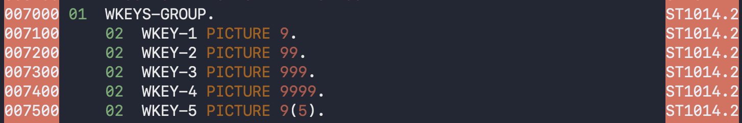
Here’s an example of a declaration in COBOL, taken from the NIST suite
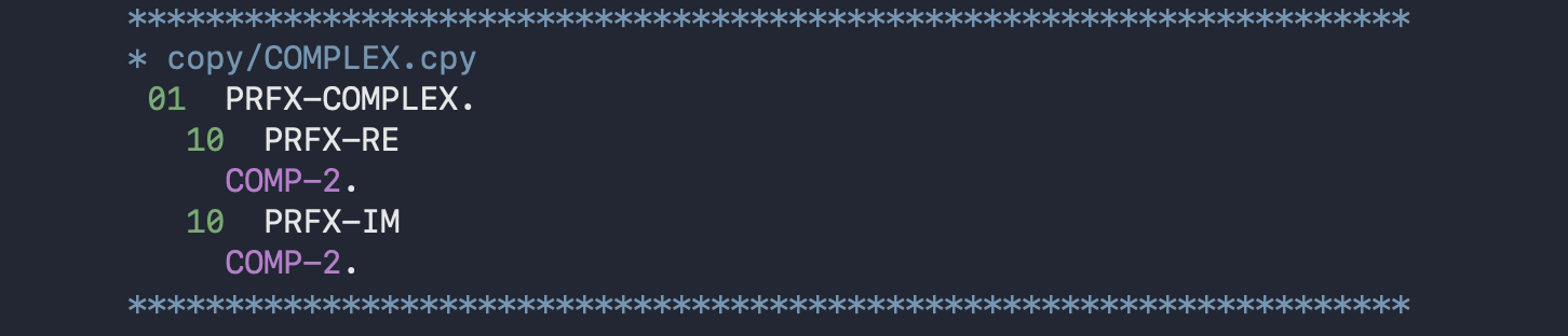
If you want a second instance of such a variable, you have to copy this and give every symbol a different name. That’s such a common pattern in COBOL that the #include like statement (COPY) has a REPLACING keyword that can be used to change a boilerplate prefix or suffix into a name that is specific to the new use. Here’s an example of a copybook fragment that is meant to be used with COPY REPLACING:
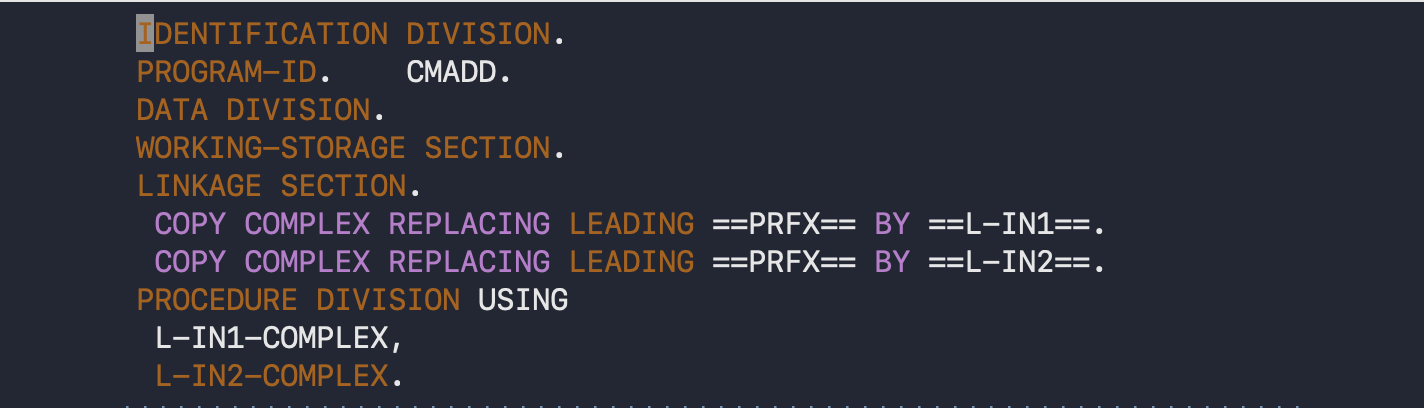
where the #include site may look like:
and the result, after preprocessing, would be:
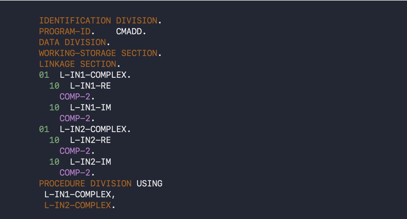
When you have two instances of the same type in COBOL, you have no way of knowing if that’s the case. There’s no real type information — instead, you have to know that the membership is all identical. For large structures, this can be very unintuitive, to say the least.
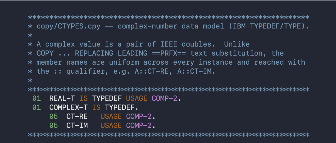
Enterprise COBOL 6.5 provides the TYPEDEF mechanism taken from TypeCOBOL & MicroFocus (according to Claude.) Instead of a COPYbook that has to be copied with REPLACING, to define a type, one can do so in a structured fashion. Example:
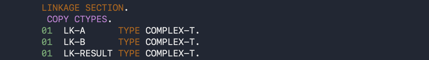
And at the use point:
Unlike conventional COBOL where every instance of “the same type” has a different name and different member names, this new declaration mechanism gives the same name to each member. You can do that in conventional COBOL, and write something like:

but this new COBOL TYPEDEF comes with a (double-colon) qualified member access syntax. Here’s an example:

Conventional COBOL qualified access would look like:

with verbosity that obscures any meaning, typical of most COBOL code. In this specific case, since the COPY REPLACING guaranteed different names for all fields, the use case could have implied membership access:

If you go looking for L-IN1-RE or L-IN2-RE, you will never find it, because it exists only as a member of the copybook that has been processed with REPLACING. This is a great example of a COBOL software development problem. Even when you have the COBOL source code, understanding the code is a reverse engineering exercise.
This TYPE/TYPEDEF syntax is nice, but it’s really just syntactic sugar. It doesn’t actually introduce any notion of strict typing to the language.
There are some minor exceptions to this lack of type safety. For example gcobol will not permit ZERO to be assigned to USAGE POINTER type. Instead you have to assign NULL. However, for the most part you can still convert anything to anything, and most of the time you’ll never get any sort of warning or error for doing so.
Despite the weak nature of this type mechanism, I think that it’s actually a very important feature. When you have a typical production COBOL program with 10000 lines of global variables (WORKING-STORAGE), you now have the capability of running an analysis that retroactively extracts the underlying implicit type representation, only known to the original programmers long since dead. You can now assign names to types that are common to a given program, and even better, names to entities that are common to a software suite. The act of reverse engineering COBOL program behaviour from the source code can then be made a little bit easier.
It only took 65 years to jam this little bit of sanity into the COBOL programming language.
User Defined Functions
The next little bit of sanity added to the language is a mechanism to define a function. If you say, wait a sec, no programming language doesn’t have functions, are you sure that COBOL doesn’t have functions.
IBM’s Enterprise COBOL 6.4, released in 2022 (according to Claude), added user defined functions, so how does this differ from the other function like constructs available in COBOL? A COBOL programmer may characterize the COBOL paragraph as a function. You can call such a “function” using the PERFORM statement. Here’s an example of a paragraph IN-4, called twice in the paragraph IN-3:
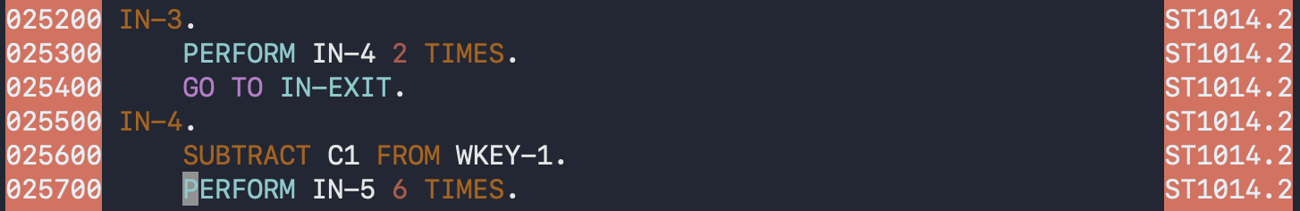
There’s a key observation to make here. Notice how the caller does not pass any parameter to the callee. That’s not just because this particular “function” takes no parameters, but it’s because that it NOT POSSIBLE to pass parameters. COBOL paragraphs are only function like in that they can be called, but
- they cannot pass parameters,
- cannot return anything,
- cannot have local variables,
- and may or may not, depending on the whim of the author, implicitly fall through to whatever code happens to follow them.
That last point is probably why, in this case, that there is a GO TO. Without that GO TO, the IN-4 paragraph may actually be executed twice. But you can’t actually know if that will be the case unless you know how you got to IN-3. If IN-3 was “called” implicitly, due to IN-2 before it finishing and falling through, then that same loop of two could be performed by:
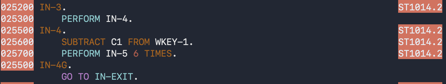
In that case, IN-4 will be executed once by IN-3, then IN-3 will fall through to IN-4 and it will execute a second time. The tricky thing about this example is that you can’t look at this code and know how many times IN-4 will be called. If IN-3 was called with PERFORM, then IN-4 will be called once, but if IN-3 was “called” by fall-through or GO TO, then IN-4 will be called twice.
Basically, the language, and all programs written in it, are sufficient to make any programmer have a terrible, horrible, no good, very bad day.
Given that paragraphs are “functions” that cannot have parameters, nor return codes, then how is is justifiable to call them functions. That justification is only possible because you can use global variables to simulate parameters and returns. Here’s an example:
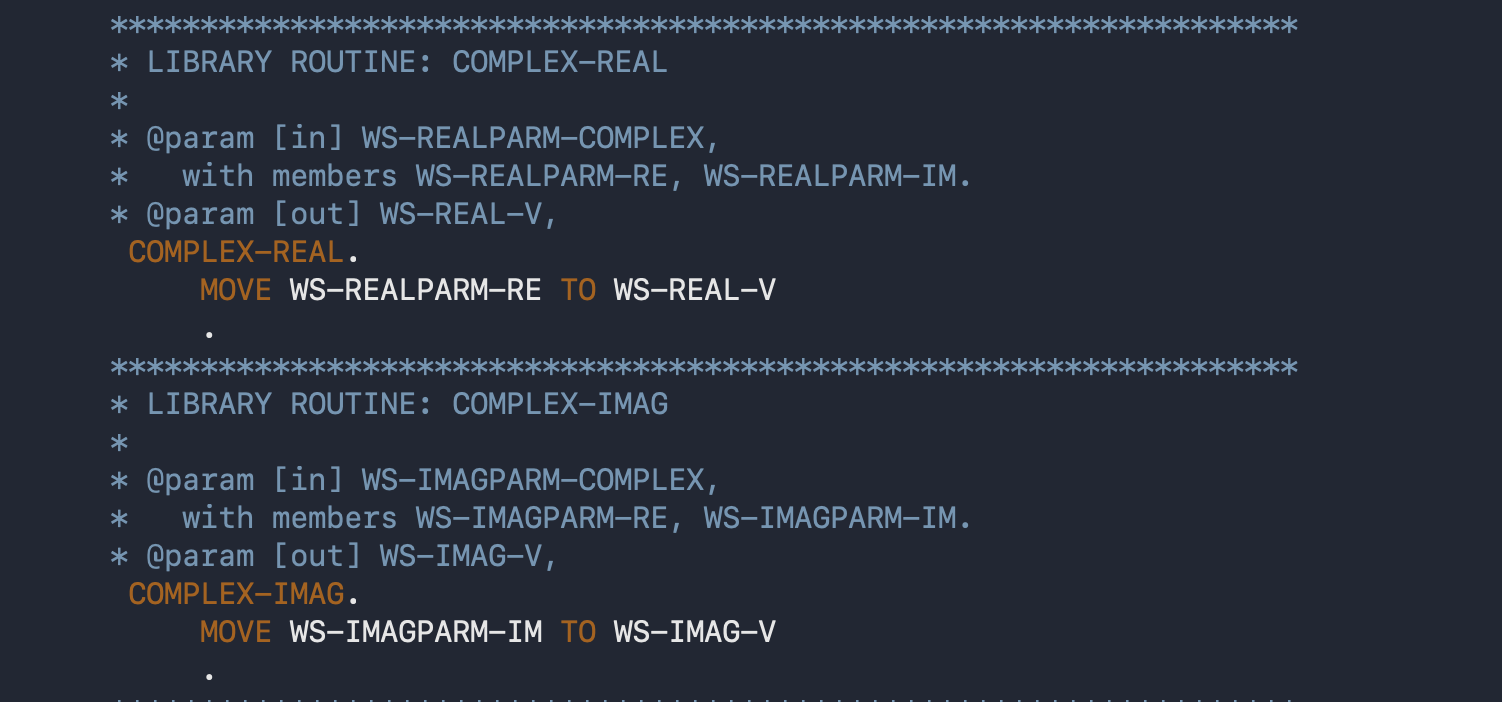
These are real and imaginary complex “functions”, each relying on you to copy values into specific “input” global variables, and get “return” values from specific output global variables.
What you will often see in production code is that programmers use naming conventions to simulate parameters, perhaps like this, for example:
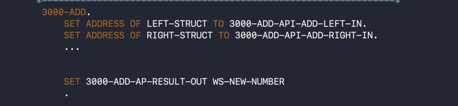
A naming convention like PARAGRAPH-<something>-IN, and PARAGRAPH-<something>-OUT, can make it more obvious that the expected use case for the code is to MOVE things to the -IN variables before a PERFORM and to grab stuff out of the -OUT variables when it’s done. You don’t have any guarantee that this is anything more than a naming convention, and any paragraph or section could potentially change the “parameter” and “return” variables of any other paragraph or section (a section is a collection of one or more paragraphs).
It is at least conceptually possible to take a well structured COBOL program, that uses a naming convention like this to model parameters, and translate it to a sane language — but you need an audit to make sure that the convention is actually followed before any sort of automatic translation can occur. And even if a program follows a function like naming convention like this, that doesn’t mean that each one, doesn’t also have a thousand other side effects that have to be figured out. With all variables usually accessed without qualification, it is very hard to look at COBOL code and have any sort of idea what data structures it is operating on.
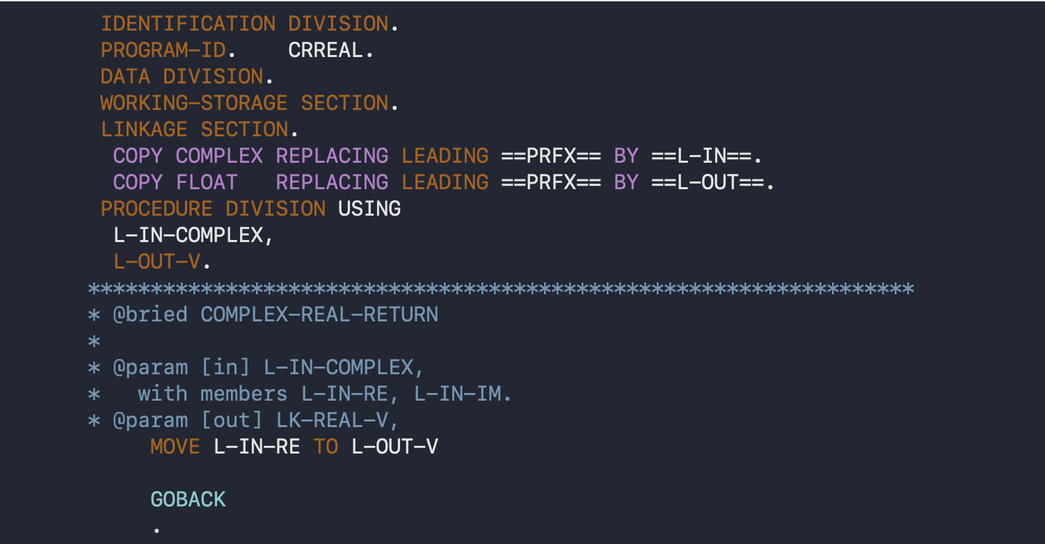
Somebody that knows COBOL may ask. What about nested subprograms and external program calls. Aren’t those “function” like. That I would agree with. A subprogram or external program is very much like a void function that passes parameters all by reference. When used in a structured way, this could model function in a modern programming language that has a set of inputs and a set of outputs, or input, outputs and mixed ins/outs.
Here’s an example of that, using the COMPLEX-REAL example above:
This might be equivalent to the following C++:
struct complex{
   double re_;
   double im_;
};

void crreal(complex * in, double * out) {
   *out = in->re_;
}
You could think of this as a function with a return *out, where *in is agreed to be used in a read only fashion.
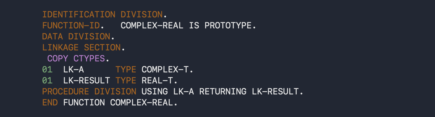
As an abstract entity, the UDF has the characteristics of a PROGRAM, specifying a FUNCTION-ID instead of a PROGRAM-ID, and also requiring a RETURNS. One might look like:
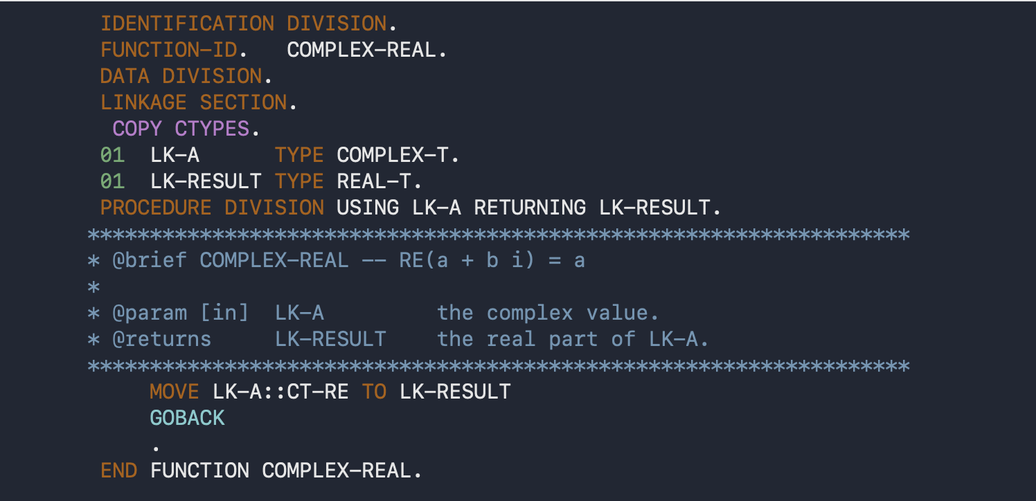
This is probably not an ideal recoding in as a UDF, as it is possible to use BY VALUE parameter passing (and I assume BY VALUE return). However, it illustrates the rough idea. One of the other differences between the UDF and a program (or subprogram) is that a UDF can be prototyped. Here’s an example of that:
Typical of COBOL, the verbosity is horrendous. This isn’t a one like prototype like you would have in C, and is much harder to read and understand. You can, however, put all the bloated PROTOTYPEs for your library functions in a copybook, and have your program COPY that. The fact that it can be prototyped is a big improvement over a COBOL program, which is completely untyped. You can have a COBOL program that takes an int by value, but pass it a parameter by reference, or vice-versa ; or that is supposed to take 3 parameters, but is passed only one, or is passed 5. The call site has no way of knowing if the type or nature of the parameters matches the implementation.
With a program being far superior to a paragraph as a function-like entity, you have to wonder why it is not a common COBOL paradigm. I suspect that a big part of that is the expense of a paragraph vs. a PROGRAM.
At LzLabs, a call to a program, subprogram or otherwise, was not cheap. A big part of that was WORKING-STORAGE related. WORKING-STORAGE is something like static storage in C, if static storage persisted across multiple invocations of a program (until “rununit” termination). Contrast that to LOCAL-STORAGE which is more “stack” like. I don’t know whether an IBM Enterprise COBOL subprogram call is any cheaper than a call to an entry function. It was not typical to see customer code that made use of PROGRAMs as function calls, except for very specific use cases.
I also don’t know if the new IBM User Defined Functions are cheap enough that programmers would opt to use them instead of paragraphs. I saw only one or two programs out of thousands (both from one customer) that used this feature, but it was still a very new feature, and relative to the age of COBOL, it still is.
At least conceivably, a UDF that doesn’t use WORKING-STORAGE (only LOCAL-STORAGE and LINKAGE-SECTION), and if used only with pass by value parameters, could, theoretically, be as cheap as a C function call. I don’t know if that’s the case on the mainframe, but it’s at least possible. You could imagine a “fastcall” convention with pass by registers for the parameters for a UDF, instead of the usual indirect “PARM” mechanism. Regardless of the cost, you could use this tomodel procedural programming in a way that can be translated to another language.
You could imagine that it would be possible to find paragraphs for which a set of WORKING-STORAGE variables are always re-written when the paragraph is executed (i.e.: find the set of variables that are effectively local to a paragraph), and then factor a paragraph out into a UDF with well defined semantics, with inputs, outputs, and local variables, reducing that giant set of “10000” working storage variables in the original program. If you repeat that process across an entire program, also extracting named representations for the implicit types used, would you be able to systematically “find” the structure of the program, and then have a candidate for translation to something not as intrinsically evil as COBOL?

