[Click here for a PDF of this post with nicer formatting]
Disclaimer
Peeter’s lecture notes from class. These may be incoherent and rough.
Matrix norm
We’ve defined the matrix norm of \( M \), for the system \( \overline{{y}} = M \overline{{x}} \) as
\begin{equation}\label{eqn:multiphysicsL6:21}
\Norm{M} = \max_{\Norm{\overline{{x}}} = 1} \Norm{ M \overline{{x}} }.
\end{equation}
We will typically use the \( L_2 \) norm, so that the matrix norm is
\begin{equation}\label{eqn:multiphysicsL6:41}
\Norm{M}_2 = \max_{\Norm{\overline{{x}}}_2 = 1} \Norm{ M \overline{{x}} }_2.
\end{equation}
It can be shown that
\begin{equation}\label{eqn:multiphysicsL6:61}
\Norm{M}_2 = \max_i \sigma_i(M),
\end{equation}
where \( \sigma_i(M) \) are the (SVD) singular values.
Singular value decomposition (SVD)
Given \( M \in R^{m \times n} \), we can find a representation of \( M \)
\begin{equation}\label{eqn:multiphysicsL6:81}
M = U \Sigma V^\T,
\end{equation}
where \( U \) and \( V\) are orthogonal matrices such that \( U^\T U = 1 \), and \( V^\T V = 1 \), and
\begin{equation}\label{eqn:multiphysicsL6:101}
\Sigma =
\begin{bmatrix}
\sigma_1 & & & & & &\\
& \sigma_2 & & & & &\\
& & \ddots & & & &\\
& & & \sigma_r & & &\\
& & & & 0 & & \\
& & & & & \ddots & \\
& & & & & & 0 \\
\end{bmatrix}
\end{equation}
The values \( \sigma_i, i \le \min(n,m) \) are called the singular values of \( M \). The singular values are subject to the ordering
\begin{equation}\label{eqn:multiphysicsL6:261}
\sigma_{1} \ge \sigma_{2} \ge \cdots \ge 0
\end{equation}
If \(r\) is the rank of \( M \), then the \( \sigma_r \) above is the minimum non-zero singular value (but the zeros are also called singular values).
Observe that the condition \( U^\T U = 1 \) is a statement of orthonormality. In terms of column vectors \( \overline{{u}}_i \), such a product written out explicitly is
\begin{equation}\label{eqn:multiphysicsL6:301}
\begin{bmatrix}
\overline{{u}}_1^\T \\ \overline{{u}}_2^\T \\ \vdots \\ \overline{{u}}_m^\T
\end{bmatrix}
\begin{bmatrix}
\overline{{u}}_1 & \overline{{u}}_2 & \cdots & \overline{{u}}_m
\end{bmatrix}
=
\begin{bmatrix}
1 & & & \\
& 1 & & \\
& & \ddots & \\
& & & 1
\end{bmatrix}.
\end{equation}
This is both normality \( \overline{{u}}_i^\T \overline{{u}}_i = 1 \), and orthonormality \( \overline{{u}}_i^\T \overline{{u}}_j = 1, i \ne j \).
Example: 2 x 2 case
(for column vectors \( \overline{{u}}_i, \overline{{v}}_j \)).
\begin{equation}\label{eqn:multiphysicsL6:281}
M =
\begin{bmatrix}
\overline{{u}}_1 & \overline{{u}}_2
\end{bmatrix}
\begin{bmatrix}
\sigma_1 & \\
& \sigma_2
\end{bmatrix}
\begin{bmatrix}
\overline{{v}}_1^\T \\
\overline{{v}}_2^\T
\end{bmatrix}
\end{equation}
Consider \( \overline{{y}} = M \overline{{x}} \), and take an \( \overline{{x}} \) with \( \Norm{\overline{{x}}}_2 = 1 \)
Note: I’ve chosen not to sketch what was drawn on the board. See instead the animated gif of the same in \citep{wiki:svd}.
A very nice video treatment of SVD by Prof Gilbert Strang can be found in \citep{ocw:svd}.
Conditioning number
Given a perturbation of \( M \overline{{x}} = \overline{{b}} \) to
\begin{equation}\label{eqn:multiphysicsL6:121}
\lr{ M + \delta M }
\lr{ \overline{{x}} + \delta \overline{{x}} } = \overline{{b}},
\end{equation}
or
\begin{equation}\label{eqn:multiphysicsL6:141}
\underbrace{ M \overline{{x}} – \overline{{b}} }_{=0} + \delta M \overline{{x}} + M \delta \overline{{x}} + \delta M \delta \overline{{x}} = 0.
\end{equation}
This gives
\begin{equation}\label{eqn:multiphysicsL6:161}
M \delta \overline{{x}} = – \delta M \overline{{x}} – \delta M \delta \overline{{x}},
\end{equation}
or
\begin{equation}\label{eqn:multiphysicsL6:181}
\delta \overline{{x}} = – M^{-1} \delta M \lr{ \overline{{x}} + \delta \overline{{x}} }.
\end{equation}
Taking norms
\begin{equation}\label{eqn:multiphysicsL6:201}
\Norm{ \delta \overline{{x}}}_2 = \Norm{
M^{-1} \delta M \lr{ \overline{{x}} + \delta \overline{{x}} }
}_2
\le
\Norm{ M^{-1} }_2 \Norm{ \delta M }_2 \Norm{ \overline{{x}} + \delta \overline{{x}} }_2,
\end{equation}
or
\begin{equation}\label{eqn:multiphysicsL6:221}
\underbrace{ \frac{\Norm{ \delta \overline{{x}}}_2 }{ \Norm{ \overline{{x}} + \delta \overline{{x}}}_2 } }_{\text{relative error of solution}}
\le
\underbrace{ \Norm{M}_2 \Norm{M^{-1}}_2 }_{\text{conditioning number of \(M\)}}
\underbrace{ \frac{ \Norm{ \delta M}_2 } {\Norm{M}_2} }_{\text{relative perturbation of \( M \)}}.
\end{equation}
The conditioning number can be shown to be
\begin{equation}\label{eqn:multiphysicsL6:241}
\text{cond}(M) =
\frac
{\sigma_{\mathrm{max}}}
{\sigma_{\mathrm{min}}}
\ge 1
\end{equation}
FIXME: justify.
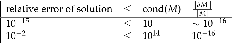
sensitivity to conditioning number
Double precision relative rounding errors can be of the order \( 10^{-16} \sim 2^{-54} \), which allows us to gauge the relative error of the solution