[Click here for a PDF of this post with nicer formatting]
Disclaimer
Peeter’s lecture notes from class. These may be incoherent and rough.
Struts and Joints, Node branch formulation
Let’s consider the simple strut system of fig. 1 again.
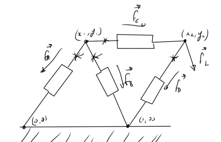
fig. 1. Simple strut system
Our unknowns are
- Forces at each of the points we have a force with two components
\begin{equation}\label{eqn:multiphysicsL12:20}
\Bf_A = \lr{ f_{A,x}, f_{A,y} }
\end{equation}We construct a total force vector\begin{equation}\label{eqn:multiphysicsL12:40}
\Bf =
\begin{bmatrix}
f_{A,x} \\
f_{A,y} \\
f_{B,x} \\
f_{B,y} \\
\vdots
\end{bmatrix}
\end{equation}
- Positions of the joints\begin{equation}\label{eqn:multiphysicsL12:60}
\Br =
\begin{bmatrix}
x_1 \\
y_1 \\
y_1 \\
y_2 \\
\vdots
\end{bmatrix}
\end{equation}
Our given variables are
- The load force \( \Bf_L \).
- The joint positions at rest.
- parameter of struts.
Conservation laws
The conservation laws are
\begin{equation}\label{eqn:multiphysicsL12:80}
\Bf_A + \Bf_B + \Bf_C = 0
\end{equation}
\begin{equation}\label{eqn:multiphysicsL12:100}
-\Bf_C + \Bf_D + \Bf_L = 0
\end{equation}
which we can put in matrix form
\begin{equation}\label{eqn:multiphysicsL12:120}
\begin{bmatrix}
1 & 0 & 1 & 0 & 1 & 0 & 0 & 0 \\
0 & 1 & 0 & 1 & 0 & 0 & 0 & 0 \\
0 & 0 & 0 & 0 & -1 & 0 & 1 & 0 \\
0 & 1 & 0 & 1 & 0 & -1 & 0 & 1 \\
\end{bmatrix}
\begin{bmatrix}
f_{A,x} \\
f_{A,y} \\
f_{B,x} \\
f_{B,y} \\
f_{C,x} \\
f_{C,y} \\
f_{D,x} \\
f_{D,y}
\end{bmatrix}
=
\begin{bmatrix}
0 \\
0 \\
-f_{L,x} \\
-f_{L,y}
\end{bmatrix}
\end{equation}
Here the block matrix is called the incidence matrix \( \BA \), and we write
\begin{equation}\label{eqn:multiphysicsL12:160}
A \Bf = \Bf_L.
\end{equation}
Constitutive laws
Given a pair of nodes as in fig. 2.
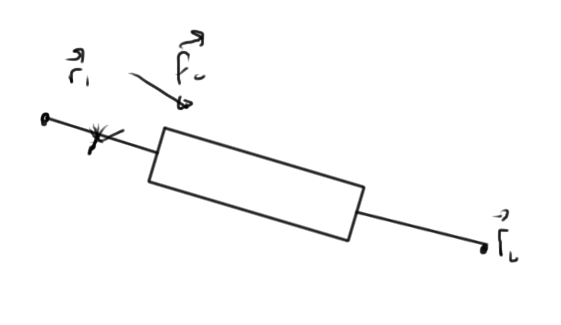
fig. 2. Strut spanning nodes
each component has an equation relating the reaction forces of that strut based on the positions
\begin{equation}\label{eqn:multiphysicsL12:180}
f_{c,x} = S_x \lr{ x_1 – x_2, y_1 – y_2, p_c }
\end{equation}
\begin{equation}\label{eqn:multiphysicsL12:200}
f_{c,y} = S_y \lr{ x_1 – x_2, y_1 – y_2, p_c },
\end{equation}
where \( p_c \) represent the parameters of the system. We write
\begin{equation}\label{eqn:multiphysicsL12:220}
\Bf =
\begin{bmatrix}
f_{A,x} \\
f_{A,y} \\
f_{B,x} \\
f_{B,y} \\
\vdots
\end{bmatrix}
=
\begin{bmatrix}
S_x \lr{ x_1 – x_2, y_1 – y_2, p_c } \\
S_y \lr{ x_1 – x_2, y_1 – y_2, p_c } \\
\vdots
\end{bmatrix},
\end{equation}
or
\begin{equation}\label{eqn:multiphysicsL12:260}
\Bf = S(\Br)
\end{equation}
Putting the pieces together
The node branch formulation is
\begin{equation}\label{eqn:multiphysicsL12:280}
\begin{aligned}
A \Bf – \Bf_L &= 0 \\
\Bf – S(\Br) &= 0
\end{aligned}
\end{equation}
We’ll want to approximate this system using the Jacobian methods discussed, and can expect the cost of that Jacobian calculation to potentially be expensive. To move to the nodal formulation we eliminate forces (the equivalent of currents in this system)
\begin{equation}\label{eqn:multiphysicsL12:320}
A S(\Br) – \Bf_L = 0
\end{equation}
We cannot use this nodal formulation when we have struts that are so stiff that the positions of some of the nodes are fixed, but can work around that as before by introducing an additional unknown for each component of such a strut.
Damped Newton’s method
We want to be able to deal with the oscillation that we can have in examples like that of fig. 3.
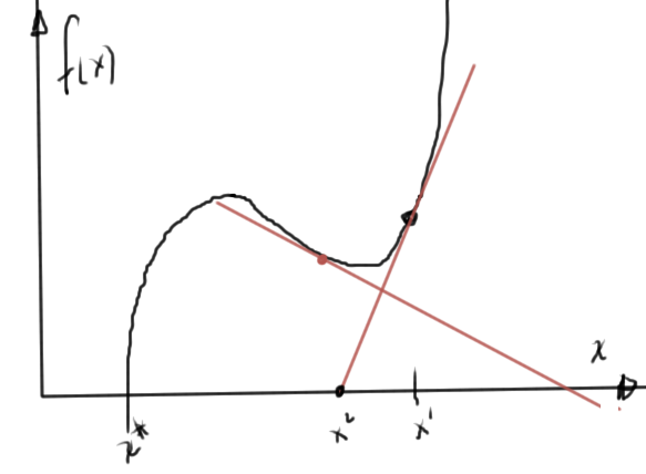
fig. 3. Oscillatory Newton’s iteration
Large steps can be dangerous. We want to modify Newton’s method as follows
Our algorithm is
- Guess \( \Bx^0, k = 0 \).
- REPEAT
- Compute \( F \) and \( J_F \) at \( \Bx^k \)
- Solve linear system \( J_F(\Bx^k) \Delta \Bx^k = – F(\Bx^k) \)
- \( \Bx^{k+1} = \Bx^k + \alpha^k \Delta \Bx^k \)
- \( k = k + 1 \)
- UNTIL converged
with \( \alpha^k = 1 \) we have standard Newton’s method. We want to pick \( \alpha^k \) so that we minimize
Continuation parameters
Newton’s method converges given a close initial guess. We can generate a sequence of problems where the previous problem generates a good initial guess for the next problem.
An example is a heat conducting bar, with a final heat distribution. We can start the numeric iteration with \( T = 0 \), and gradually increase the temperatures until we achieve the final desired heat distribution.
Suppose that we want to solve
\begin{equation}\label{eqn:multiphysicsL12:340}
F(\Bx) = 0.
\end{equation}
We modify this problem by introducing
\begin{equation}\label{eqn:multiphysicsL12:360}
\tilde{F}(\Bx(\lambda), \lambda) = 0,
\end{equation}
where
- \( \tilde{F}(\Bx(0), 0) = 0 \) is easy to solve
- \( \tilde{F}(\Bx(1), 1) = 0 \) is equivalent to \( F(\Bx) = 0 \).
- (more on slides)
The source load stepping algorithm is
- Solve \(\tilde{F}(\Bx(0), 0) = 0 \), with \( \Bx(\lambda_{\text{prev}} = \Bx(0) \)
- (more on slides)
This can still have problems, for example, when the parameterization is multivalued as in fig. 4.
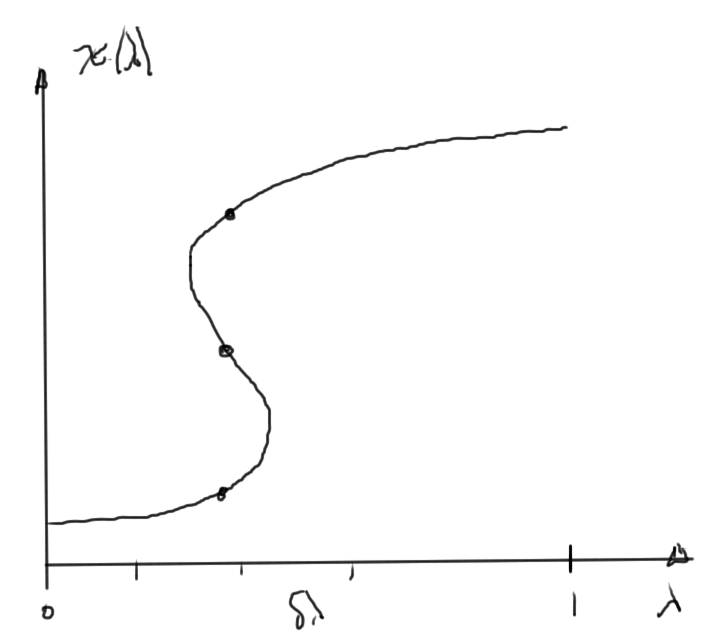
fig. 4. Multivalued parameterization
We can attempt to adjust \( \lambda \) so that we move along the parameterization curve.