[Click here for a PDF of this post with nicer formatting]
Disclaimer
Peeter’s lecture notes from class. These may be incoherent and rough.
Singular Jacobians
(mostly on slides)
There is the possiblity of singular Jacobians to consider. FIXME: not sure how this system represented that. Look on slides.
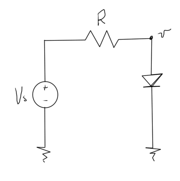
fig. 1. Diode system that results in singular Jacobian
\begin{equation}\label{eqn:multiphysicsL13:20}
\tilde{f}(v(\lambda), \lambda) = i(v) – \inv{R}( v – \lambda V_s ) = 0.
\end{equation}
An alternate continuation scheme uses
\begin{equation}\label{eqn:multiphysicsL13:40}
\tilde{F}(\Bx(\lambda), \lambda) = \lambda F(\Bx(\lambda)) + (1-\lambda) \Bx(\lambda).
\end{equation}
This scheme has
\begin{equation}\label{eqn:multiphysicsL13:60}
\tilde{F}(\Bx(0), 0) = 0
\end{equation}
\begin{equation}\label{eqn:multiphysicsL13:80}
\tilde{F}(\Bx(1), 1) = F(\Bx(1)),
\end{equation}
and for one variable, easy to compute Jacobian at the origin, or the original Jacobian at \( \lambda = 1 \)
\begin{equation}\label{eqn:multiphysicsL13:100}
\PD{x}{\tilde{F}}(x(0), 0) = I
\end{equation}
\begin{equation}\label{eqn:multiphysicsL13:120}
\PD{x}{\tilde{F}}(x(1), 1) = \PD{x}{F}(x(1))
\end{equation}
Simulation of dynamical systems
Example high level system in fig. 2.
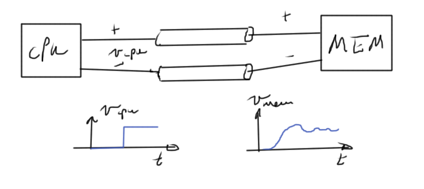
fig. 2. Complex time dependent system
Assembling equations automatically for dynamical systems
RC circuit
To demonstrate the method by example consider the RC circuit fig. 3 which has time dependence that must be considered
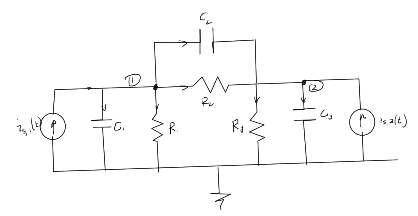
fig. 3. RC circuit
The unknowns are \( v_1(t), v_2(t) \).
The equations (KCLs) at each of the nodes are
- \(
\frac{v_1(t)}{R_1}
+ C_1 \frac{dv_1}{dt}
+ \frac{v_1(t) – v_2(t)}{R_2}
+ C_2 \frac{d(v_1 – v_2)}{dt}
– i_{s,1}(t) = 0
\) - \(
\frac{v_2(t) – v_1(t)}{R_2}
+ C_2 \frac{d(v_2 – v_1)}{dt}
+ \frac{v_2(t)}{R_3}
+ C_3 \frac{dv_2}{dt}
– i_{s,2}(t)
= 0
\)
This has the matrix form
\begin{equation}\label{eqn:multiphysicsL13:140}
\begin{bmatrix}
Z_1 + Z_2 & – Z_2 \\
-Z_2 & Z_2 + Z_3
\end{bmatrix}
\begin{bmatrix}
v_1(t) \\
v_2(t)
\end{bmatrix}
+
\begin{bmatrix}
C_1 + C_2 & -C_2 \\
– C_2 & C_2 + C_3
\end{bmatrix}
\begin{bmatrix}
\frac{dv_1(t)}{dt} \\
\frac{dv_2(t}{dt})
\end{bmatrix}
=
\begin{bmatrix}
1 & 0 \\
0 & 1
\end{bmatrix}
\begin{bmatrix}
i_{s,1}(t) \\
i_{s,2}(t)
\end{bmatrix}.
\end{equation}
Observe that the capacitor between node 2 and 1 is associated with a stamp of the form
\begin{equation}\label{eqn:multiphysicsL13:180}
\begin{bmatrix}
C_2 & -C_2 \\
-C_2 & C_2
\end{bmatrix},
\end{equation}
very much like the impedance stamps of the resistor node elements.
The RC circuit problem has the abstract form
\begin{equation}\label{eqn:multiphysicsL13:160}
G \Bx(t) + C \frac{d\Bx(t)}{dt} = B \Bu(t),
\end{equation}
which is more general than a state space equation of the form
\begin{equation}\label{eqn:multiphysicsL13:200}
\frac{d\Bx(t)}{dt} = A \Bx(t) + B \Bu(t).
\end{equation}
Such a system may be represented diagramatically as in fig. 4.
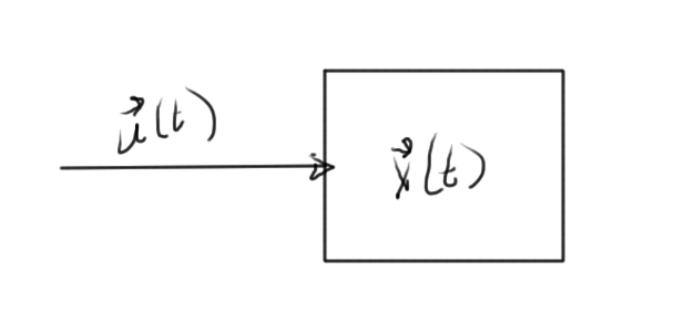
fig. 4. State space system
The \( C \) factor in this capacitance system, is generally not invertable. For example, if consider a 10 node system with only one capacitor, for which \( C \) will be mostly zeros.
In a state space system, in all equations we have a derivative. All equations are dynamical.
The time dependent MNA system for the RC circuit above, contains a mix of dynamical and algebraic equations. This could, for example, be a pair of equations like
\begin{equation}\label{eqn:multiphysicsL13:240}
\frac{dx_1}{dt} + x_2 + 3 = 0
\end{equation}
\begin{equation}\label{eqn:multiphysicsL13:260}
x_1 + x_2 + 3 = 0
\end{equation}
How to handle inductors
A pair of nodes that contains an inductor element, as in fig. 5, has to be handled specially.
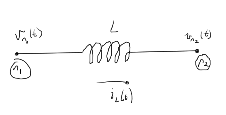
fig. 5. Inductor configuration
The KCL at node 1 has the form
\begin{equation}\label{eqn:multiphysicsL13:280}
\cdots + i_L(t) + \cdots = 0,
\end{equation}
where
\begin{equation}\label{eqn:multiphysicsL13:300}
v_{n_1}(t) – v_{n_2}(t) = L \frac{d i_L}{dt}.
\end{equation}
It is possible to express this in terms of \( i_L \), the variable of interest
\begin{equation}\label{eqn:multiphysicsL13:320}
i_L(t) = \inv{L} \int_0^t \lr{ v_{n_1}(\tau) – v_{n_2}(\tau) } d\tau
+ i_L(0).
\end{equation}
Expressing the problem directly in terms of such integrals makes the problem harder to solve, since the usual differential equation toolbox cannot be used directly. An integro-differential toolbox would have to be developed. What can be done instead is to introduce an additional unknown for each inductor current derivative \( di_L/dt \), for which an additional MNA row is introduced for that inductor scaled voltage difference.
Numerical solution of differential equations
Consider the one variable system
\begin{equation}\label{eqn:multiphysicsL13:340}
G x(t) + C \frac{dx}{dt} = B u(t),
\end{equation}
given an initial condition \( x(0) = x_0 \). Imagine that this system has the solution sketched in fig. 6.
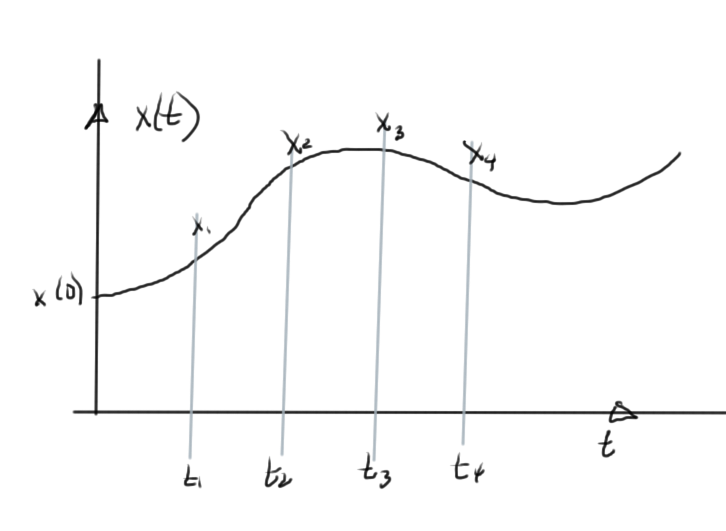
fig. 6. Discrete time sampling
Very roughly, the steps for solution are of the form
- Discretize time
- Aim to find the solution at \( t_1, t_2, t_3, \cdots \)
- Use a finite difference formula to approximate the derivative.
There are various schemes that can be used to discretize, and compute the finite differences.
Forward Euler method
\index{forward Euler method}
One such scheme is to use the forward differences, as in fig. 7, to approximate the derivative
\begin{equation}\label{eqn:multiphysicsL13:360}
\dot{x}(t_n) \approx \frac{x_{n+1} – x_n}{\Delta t}.
\end{equation}
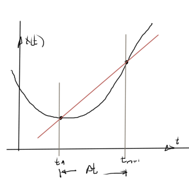
fig. 7. Forward difference derivative approximation
Introducing this into \ref{eqn:multiphysicsL13:340} gives
\begin{equation}\label{eqn:multiphysicsL13:350}
G x_n + C \frac{x_{n+1} – x_n}{\Delta t} = B u(t_n),
\end{equation}
or
\begin{equation}\label{eqn:multiphysicsL13:380}
C x_{n+1} = \Delta t B u(t_n) – \Delta t G x_n + C x_n.
\end{equation}
The coefficient \( C \) must be invertable, and the next point follows immediately
\begin{equation}\label{eqn:multiphysicsL13:381}
x_{n+1} = \frac{\Delta t B}{C} u(t_n)
+ x_n \lr{ 1 – \frac{\Delta t G}{C} }.
\end{equation}