[Click here for a PDF of this post with nicer formatting]
Disclaimer
Peeter’s lecture notes from class. These may be incoherent and rough.
These are notes for the UofT course ECE1505H, Convex Optimization, taught by Prof. Stark Draper.
Matrix inner product
Given real matrices \( X, Y \in \mathbb{R}^{m\times n} \), one possible matrix inner product definition is
\begin{equation}\label{eqn:convexOptimizationLecture3:20}
\begin{aligned}
\innerprod{X}{Y}
&= \textrm{Tr}( X^\T Y) \\
&= \textrm{Tr} \lr{ \sum_{k = 1}^m X_{ki} Y_{kj} } \\
&= \sum_{k = 1}^m \sum_{j = 1}^n X_{kj} Y_{kj} \\
&= \sum_{i = 1}^m \sum_{j = 1}^n X_{ij} Y_{ij}.
\end{aligned}
\end{equation}
This inner product induces a norm on the (matrix) vector space, called the Frobenius norm
\begin{equation}\label{eqn:convexOptimizationLecture3:40}
\begin{aligned}
\Norm{X }_F
&= \textrm{Tr}( X^\T X) \\
&= \sqrt{ \innerprod{X}{X} } \\
&=
\sum_{i = 1}^m \sum_{j = 1}^n X_{ij}^2.
\end{aligned}
\end{equation}
Range, nullspace.
Definition: Range: Given \( A \in \mathbb{R}^{m \times n} \), the range of A is the set:
\begin{equation*}
\mathcal{R}(A) = \setlr{ A \Bx | \Bx \in \mathbb{R}^n }.
\end{equation*}
Definition: Nullspace: Given \( A \in \mathbb{R}^{m \times n} \), the nullspace of A is the set:
\begin{equation*}
\mathcal{N}(A) = \setlr{ \Bx | A \Bx = 0 }.
\end{equation*}
SVD.
To understand operation of \( A \in \mathbb{R}^{m \times n} \), a representation of a linear transformation from \R{n} to \R{m}, decompose \( A \) using the singular value decomposition (SVD).
Definition: SVD: Given \( A \in \mathbb{R}^{m \times n} \), an operator on \( \Bx \in \mathbb{R}^n \), a decomposition of the following form is always possible
\begin{equation*}
\begin{aligned}
A &= U \Sigma V^\T \\
U &\in \mathbb{R}^{m \times r} \\
V &\in \mathbb{R}^{n \times r},
\end{aligned}
\end{equation*}
where \( r \) is the rank of \(A\), and both \( U \) and \( V \) are orthogonal
\begin{equation*}
\begin{aligned}
U^\T U &= I \in \mathbb{R}^{r \times r} \\
V^\T V &= I \in \mathbb{R}^{r \times r}.
\end{aligned}
\end{equation*}
Here \( \Sigma = \textrm{diag}( \sigma_1, \sigma_2, \cdots, \sigma_r ) \), is a diagonal matrix of “singular” values, where
\begin{equation*}
\sigma_1 \ge \sigma_2 \ge \cdots \ge \sigma_r.
\end{equation*}
For simplicity consider square case \( m = n \)
\begin{equation}\label{eqn:convexOptimizationLecture3:100}
A \Bx = \lr{ U \Sigma V^\T } \Bx.
\end{equation}
The first product \( V^\T \Bx \) is a rotation, which can be checked by looking at the length
\begin{equation}\label{eqn:convexOptimizationLecture3:120}
\begin{aligned}
\Norm{ V^\T \Bx}_2
&= \sqrt{ \Bx^\T V V^\T \Bx } \\
&= \sqrt{ \Bx^\T \Bx } \\
&= \Norm{ \Bx }_2,
\end{aligned}
\end{equation}
which shows that the length of the vector is unchanged after application of the linear transformation represented by \( V^\T \) so that operation must be a rotation.
Similarly the operation of \( U \) on \( \Sigma V^\T \Bx \) also must be a rotation. The operation \( \Sigma = [\sigma_i]_i \) applies a scaling operation to each component of the vector \( V^\T \Bx \).
All linear (square) transformations can therefore be thought of as a rotate-scale-rotate operation. Often the \( A \) of interest will be symmetric \( A = A^\T \).
Set of symmetric matrices
Let \( S^n \) be the set of real, symmetric \( n \times n \) matrices.
Theorem: Spectral theorem: When \( A \in S^n \) then it is possible to factor \( A \) as
\begin{equation*}
A = Q \Lambda Q^\T,
\end{equation*}
where \( Q \) is an orthogonal matrix, and \( \Lambda = \textrm{diag}( \lambda_1, \lambda_2, \cdots \lambda_n)\). Here \( \lambda_i \in \mathbb{R} \, \forall i \) are the (real) eigenvalues of \( A \).
A real symmetric matrix \( A \in S^n\) is “positive semi-definite” if
\begin{equation*}
\Bv^\T A \Bv \ge 0 \qquad\forall \Bv \in \mathbb{R}^n, \Bv \ne 0,
\end{equation*}
and is “positive definite” if
\begin{equation*}
\Bv^\T A \Bv > 0 \qquad\forall \Bv \in \mathbb{R}^n, \Bv \ne 0.
\end{equation*}
The set of such matrices is denoted \( S^n_{+} \), and \( S^n_{++} \) respectively.
Consider \( A \in S^n_{+} \) (or \( S^n_{++} \) )
\begin{equation}\label{eqn:convexOptimizationLecture3:200}
A = Q \Lambda Q^\T,
\end{equation}
possible since the matrix is symmetric. For such a matrix
\begin{equation}\label{eqn:convexOptimizationLecture3:220}
\begin{aligned}
\Bv^\T A \Bv
&=
\Bv^\T Q \Lambda A^\T \Bv \\
&=
\Bw^\T \Lambda \Bw,
\end{aligned}
\end{equation}
where \( \Bw = A^\T \Bv \). Such a product is
\begin{equation}\label{eqn:convexOptimizationLecture3:240}
\Bv^\T A \Bv
=
\sum_{i = 1}^n \lambda_i w_i^2.
\end{equation}
So, if \( \lambda_i \ge 0 \) (\(\lambda_i > 0 \) ) then \( \sum_{i = 1}^n \lambda_i w_i^2 \) is non-negative (positive) \( \forall \Bw \in \mathbb{R}^n, \Bw \ne 0 \). Since \( \Bw \) is just a rotated version of \( \Bv \) this also holds for all \( \Bv \). A necessary and sufficient condition for \( A \in S^n_{+} \) (\( S^n_{++} \) ) is \( \lambda_i \ge 0 \) (\(\lambda_i > 0\)).
Square root of positive semi-definite matrix
Real symmetric matrix power relationships such as
\begin{equation}\label{eqn:convexOptimizationLecture3:260}
A^2
=
Q \Lambda Q^\T
Q \Lambda Q^\T
=
Q \Lambda^2
Q^\T
,
\end{equation}
or more generally \( A^k = Q \Lambda^k Q^\T,\, k \in \mathbb{Z} \), can be further generalized to non-integral powers. In particular, the square root (non-unique) of a square matrix can be written
\begin{equation}\label{eqn:convexOptimizationLecture3:280}
A^{1/2} = Q
\begin{bmatrix}
\sqrt{\lambda_1} & & & \\
& \sqrt{\lambda_2} & & \\
& & \ddots & \\
& & & \sqrt{\lambda_n} \\
\end{bmatrix}
Q^\T,
\end{equation}
since \( A^{1/2} A^{1/2} = A \), regardless of the sign picked for the square roots in question.
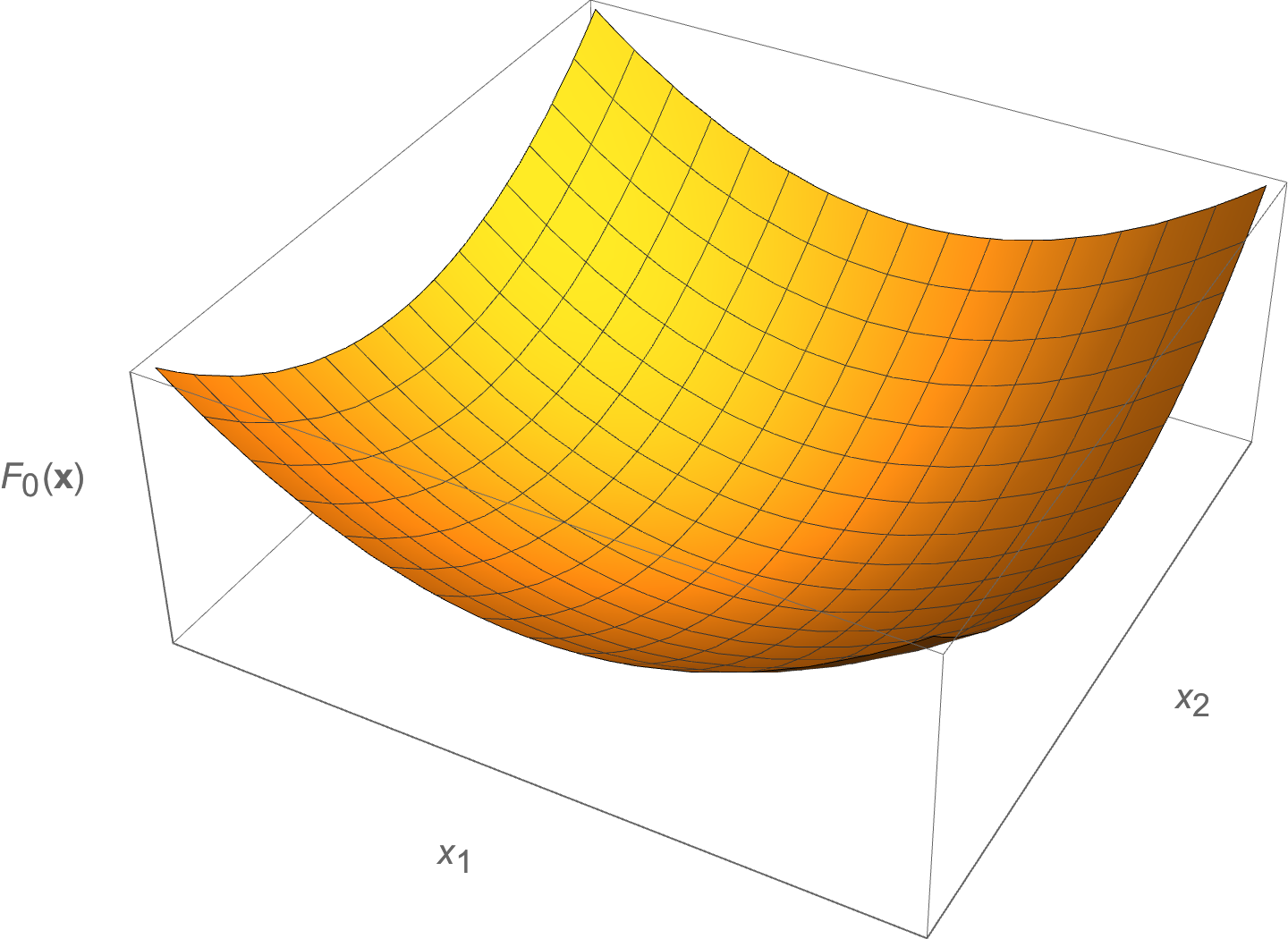
Functions of matrices
Consider \( F : S^n \rightarrow \mathbb{R} \), and define
\begin{equation}\label{eqn:convexOptimizationLecture3:300}
F(X) = \log \det X,
\end{equation}
Here \( \textrm{dom} F = S^n_{++} \). The task is to find \( \spacegrad F \), which can be done by looking at the perturbation \( \log \det ( X + \Delta X ) \)
\begin{equation}\label{eqn:convexOptimizationLecture3:320}
\begin{aligned}
\log \det ( X + \Delta X )
&=
\log \det ( X^{1/2} (I + X^{-1/2} \Delta X X^{-1/2}) X^{1/2} ) \\
&=
\log \det ( X (I + X^{-1/2} \Delta X X^{-1/2}) ) \\
&=
\log \det X + \log \det (I + X^{-1/2} \Delta X X^{-1/2}).
\end{aligned}
\end{equation}
Let \( X^{-1/2} \Delta X X^{-1/2} = M \) where \( \lambda_i \) are the eigenvalues of \( M : M \Bv = \lambda_i \Bv \) when \( \Bv \) is an eigenvector of \( M \). In particular
\begin{equation}\label{eqn:convexOptimizationLecture3:340}
(I + M) \Bv =
(1 + \lambda_i) \Bv,
\end{equation}
where \( 1 + \lambda_i \) are the eigenvalues of the \( I + M \) matrix. Since the determinant is the product of the eigenvalues, this gives
\begin{equation}\label{eqn:convexOptimizationLecture3:360}
\begin{aligned}
\log \det ( X + \Delta X )
&=
\log \det X +
\log \prod_{i = 1}^n (1 + \lambda_i) \\
&=
\log \det X +
\sum_{i = 1}^n \log (1 + \lambda_i).
\end{aligned}
\end{equation}
If \( \lambda_i \) are sufficiently “small”, then \( \log ( 1 + \lambda_i ) \approx \lambda_i \), giving
\begin{equation}\label{eqn:convexOptimizationLecture3:380}
\log \det ( X + \Delta X )
=
\log \det X +
\sum_{i = 1}^n \lambda_i
\approx
\log \det X +
\textrm{Tr}( X^{-1/2} \Delta X X^{-1/2} ).
\end{equation}
Since
\begin{equation}\label{eqn:convexOptimizationLecture3:400}
\textrm{Tr}( A B ) = \textrm{Tr}( B A ),
\end{equation}
this trace operation can be written as
\begin{equation}\label{eqn:convexOptimizationLecture3:420}
\log \det ( X + \Delta X )
\approx
\log \det X +
\textrm{Tr}( X^{-1} \Delta X )
=
\log \det X +
\innerprod{ X^{-1}}{\Delta X},
\end{equation}
so
\begin{equation}\label{eqn:convexOptimizationLecture3:440}
\spacegrad F(X) = X^{-1}.
\end{equation}
To check this, consider the simplest example with \( X \in \mathbb{R}^{1 \times 1} \), where we have
\begin{equation}\label{eqn:convexOptimizationLecture3:460}
\frac{d}{dX} \lr{ \log \det X } = \frac{d}{dX} \lr{ \log X } = \inv{X} = X^{-1}.
\end{equation}
This is a nice example demonstrating how the gradient can be obtained by performing a first order perturbation of the function. The gradient can then be read off from the result.
Second order perturbations
- To get first order approximation found the part that varied linearly in \( \Delta X \).
- To get the second order part, perturb \( X^{-1} \) by \( \Delta X \) and see how that perturbation varies in \( \Delta X \).
For \( G(X) = X^{-1} \), this is
\begin{equation}\label{eqn:convexOptimizationLecture3:480}
\begin{aligned}
(X + \Delta X)^{-1}
&=
\lr{ X^{1/2} (I + X^{-1/2} \Delta X X^{-1/2} ) X^{1/2} }^{-1} \\
&=
X^{-1/2} (I + X^{-1/2} \Delta X X^{-1/2} )^{-1} X^{-1/2}
\end{aligned}
\end{equation}
To be proven in the homework (for “small” A)
\begin{equation}\label{eqn:convexOptimizationLecture3:500}
(I + A)^{-1} \approx I – A.
\end{equation}
This gives
\begin{equation}\label{eqn:convexOptimizationLecture3:520}
\begin{aligned}
(X + \Delta X)^{-1}
&=
X^{-1/2} (I – X^{-1/2} \Delta X X^{-1/2} ) X^{-1/2} \\
&=
X^{-1} – X^{-1} \Delta X X^{-1},
\end{aligned}
\end{equation}
or
\begin{equation}\label{eqn:convexOptimizationLecture3:800}
\begin{aligned}
G(X + \Delta X)
&= G(X) + (D G) \Delta X \\
&= G(X) + (\spacegrad G)^\T \Delta X,
\end{aligned}
\end{equation}
so
\begin{equation}\label{eqn:convexOptimizationLecture3:820}
(\spacegrad G)^\T \Delta X
=
– X^{-1} \Delta X X^{-1}.
\end{equation}
The Taylor expansion of \( F \) to second order is
\begin{equation}\label{eqn:convexOptimizationLecture3:840}
F(X + \Delta X)
=
F(X)
+
\textrm{Tr} \lr{ (\spacegrad F)^\T \Delta X}
+
\inv{2}
\lr{ (\Delta X)^\T (\spacegrad^2 F) \Delta X}.
\end{equation}
The first trace can be expressed as an inner product
\begin{equation}\label{eqn:convexOptimizationLecture3:860}
\begin{aligned}
\textrm{Tr} \lr{ (\spacegrad F)^\T \Delta X}
&=
\innerprod{ \spacegrad F }{\Delta X} \\
&=
\innerprod{ X^{-1} }{\Delta X}.
\end{aligned}
\end{equation}
The second trace also has the structure of an inner product
\begin{equation}\label{eqn:convexOptimizationLecture3:880}
\begin{aligned}
(\Delta X)^\T (\spacegrad^2 F) \Delta X
&=
\textrm{Tr} \lr{ (\Delta X)^\T (\spacegrad^2 F) \Delta X} \\
&=
\innerprod{ (\spacegrad^2 F)^\T \Delta X }{\Delta X},
\end{aligned}
\end{equation}
where a no-op trace could be inserted in the second order term since that quadratic form is already a scalar. This \( (\spacegrad^2 F)^\T \Delta X \) term has essentially been found implicitly by performing the linear variation of \( \spacegrad F \) in \( \Delta X \), showing that we must have
\begin{equation}\label{eqn:convexOptimizationLecture3:900}
\textrm{Tr} \lr{ (\Delta X)^\T (\spacegrad^2 F) \Delta X}
=
\innerprod{ – X^{-1} \Delta X X^{-1} }{\Delta X},
\end{equation}
so
\begin{equation}\label{eqn:convexOptimizationLecture3:560}
F( X + \Delta X) = F(X) +
\innerprod{X^{-1}}{\Delta X}
+\inv{2} \innerprod{-X^{-1} \Delta X X^{-1}}{\Delta X},
\end{equation}
or
\begin{equation}\label{eqn:convexOptimizationLecture3:580}
\log \det ( X + \Delta X) = \log \det X +
\textrm{Tr}( X^{-1} \Delta X )
– \inv{2} \textrm{Tr}( X^{-1} \Delta X X^{-1} \Delta X ).
\end{equation}
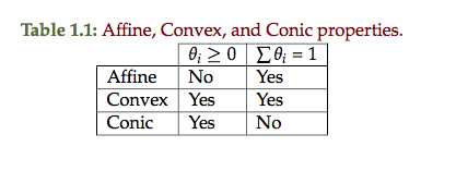
Convex Sets
- Types of sets: Affine, convex, cones
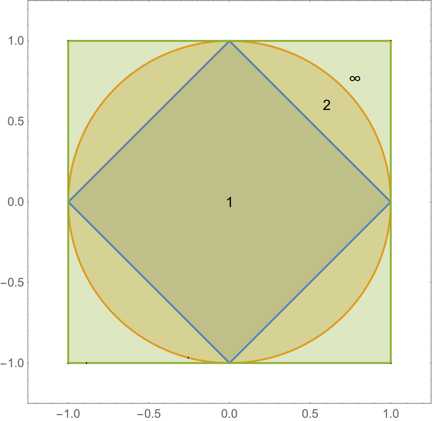
- Examples: Hyperplanes, polyhedra, balls, ellipses, norm balls, cone of PSD matrices.
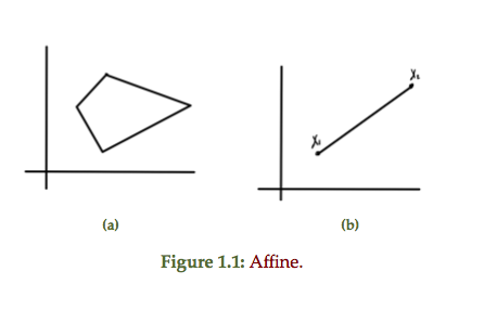
Definition: Affine set:
A set \( C \subseteq \mathbb{R}^n \) is affine if \( \forall \Bx_1, \Bx_2 \in C \) then
\begin{equation*}
\theta \Bx_1 + (1 -\theta) \Bx_2 \in C, \qquad \forall \theta \in \mathbb{R}.
\end{equation*}
The affine sum above can
be rewritten as
\begin{equation}\label{eqn:convexOptimizationLecture3:600}
\Bx_2 + \theta (\Bx_1 – \Bx_2).
\end{equation}
Since \( \theta \) is a scaling, this is the line containing \( \Bx_2 \) in the direction between \( \Bx_1 \) and \( \Bx_2 \).
Observe that the solution to a set of linear equations
\begin{equation}\label{eqn:convexOptimizationLecture3:620}
C = \setlr{ \Bx | A \Bx = \Bb },
\end{equation}
is an affine set. To check, note that
\begin{equation}\label{eqn:convexOptimizationLecture3:640}
\begin{aligned}
A (\theta \Bx_1 + (1 – \theta) \Bx_2)
&=
\theta A \Bx_1 + (1 – \theta) A \Bx_2 \\
&=
\theta \Bb + (1 – \theta) \Bb \\
&= \Bb.
\end{aligned}
\end{equation}
Definition: Affine combination: An affine combination of points \( \Bx_1, \Bx_2, \cdots \Bx_n \) is
\begin{equation*}
\sum_{i = 1}^n \theta_i \Bx_i,
\end{equation*}
such that for \( \theta_i \in \mathbb{R} \)
\begin{equation*}
\sum_{i = 1}^n \theta_i = 1.
\end{equation*}
An affine set contains all affine combinations of points in the set. Examples of a couple affine sets are sketched in fig 1.1
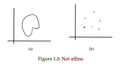
For comparison, a couple of non-affine sets are sketched in fig 1.2
Definition: Convex set: A set \( C \subseteq \mathbb{R}^n \) is convex if \( \forall \Bx_1, \Bx_2 \in C \) and \( \forall \theta \in \mathbb{R}, \theta \in [0,1] \), the combination
\begin{equation}\label{eqn:convexOptimizationLecture3:700}
\theta \Bx_1 + (1 – \theta) \Bx_2 \in C.
\end{equation}
Definition: Convex combination: A convex combination of \( \Bx_1, \Bx_2, \cdots \Bx_n \) is
\begin{equation*}
\sum_{i = 1}^n \theta_i \Bx_i,
\end{equation*}
such that \( \forall \theta_i \ge 0 \)
\begin{equation*}
\sum_{i = 1}^n \theta_i = 1
\end{equation*}
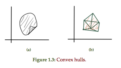
Definition: Convex hull: Convex hull of a set \( C \) is a set of all convex combinations of points in \(C\), denoted
\begin{equation}\label{eqn:convexOptimizationLecture3:720}
\textrm{conv}(C) = \setlr{ \sum_{i=1}^n \theta_i \Bx_i | \Bx_i \in C, \theta_i \ge 0, \sum_{i=1}^n \theta_i = 1 }.
\end{equation}
A non-convex set can be converted into a convex hull by filling in all the combinations of points connecting points in the set, as sketched in fig 1.3.
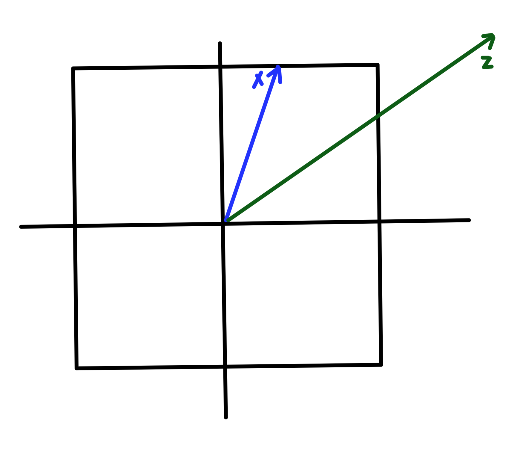
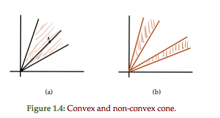
Definition: Cone: A set \(C\) is a cone if \( \forall \Bx \in C \) and \( \forall \theta \ge 0 \) we have \( \theta \Bx \in C\).
This scales out if \(\theta > 1\) and scales in if \(\theta < 1\).
A convex cone is a cone that is also a convex set. A conic combination is
\begin{equation*}
\sum_{i=1}^n \theta_i \Bx_i, \theta_i \ge 0.
\end{equation*}
A convex and non-convex 2D cone is sketched in fig. 1.4
A comparison of properties for different set types is tabulated in table 1.1
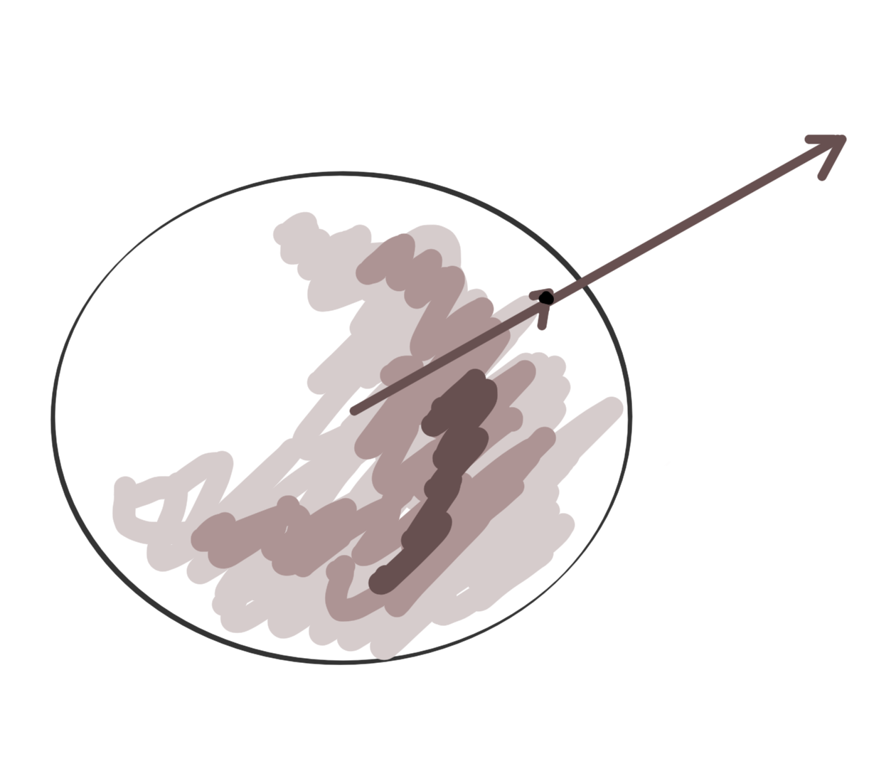
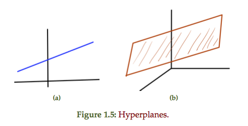
Hyperplanes and half spaces
Definition: Hyperplane: A hyperplane is defined by
\begin{equation*}
\setlr{ \Bx | \Ba^\T \Bx = \Bb, \Ba \ne 0 }.
\end{equation*}
A line and plane are examples of this general construct as sketched in
fig. 1.5
An alternate view is possible should one
find any specific \( \Bx_0 \) such that \( \Ba^\T \Bx_0 = \Bb \)
\begin{equation}\label{eqn:convexOptimizationLecture3:740}
\setlr{\Bx | \Ba^\T \Bx = b }
=
\setlr{\Bx | \Ba^\T (\Bx -\Bx_0) = 0 }
\end{equation}
This shows that \( \Bx – \Bx_0 = \Ba^\perp \) is perpendicular to \( \Ba \), or
\begin{equation}\label{eqn:convexOptimizationLecture3:780}
\Bx
=
\Bx_0 + \Ba^\perp.
\end{equation}
This is the subspace perpendicular to \( \Ba \) shifted by \(\Bx_0\), subject to \( \Ba^\T \Bx_0 = \Bb \). As a set
\begin{equation}\label{eqn:convexOptimizationLecture3:760}
\Ba^\perp = \setlr{ \Bv | \Ba^\T \Bv = 0 }.
\end{equation}
Half space
Definition: Half space: The half space is defined as
\begin{equation*}
\setlr{ \Bx | \Ba^\T \Bx = \Bb }
= \setlr{ \Bx | \Ba^\T (\Bx – \Bx_0) \le 0 }.
\end{equation*}
This can also be expressed as \( \setlr{ \Bx | \innerprod{ \Ba }{\Bx – \Bx_0 } \le 0 } \).