[Click here for a PDF version of this post]
Motivation.
Having just worked one of Karl’s problems for the distance between two parallel planes, I recalled that when I was in high school, I had trouble with the intuition for the problem of shortest distance between two lines.
In this post, I’ll revisit that ancient trouble and finally come to terms with it.
Distance from origin to a line.
Before doing the two lines problem, let’s look at a similar simpler problem, the shortest distance from the origin to a line. The parametric representation of a line going through point \( \Bp \) with (unit) direction vector \( \mathbf{\hat{d}} \) is
\begin{equation}\label{eqn:shortestDistanceBetweenLines:40}
L: \Bx(r) = \Bp + r \mathbf{\hat{d}}.
\end{equation}
If we want to solve this the dumb but mechanical way, we have only to minimize a length-squared function for the distance to a point on the line
\begin{equation}\label{eqn:shortestDistanceBetweenLines:60}
\begin{aligned}
D
&= \Norm{\Bx}^2 \\
&= \Bp^2 + r^2 + 2 r \Bp \cdot \mathbf{\hat{d}}.
\end{aligned}
\end{equation}
The minimum will occur where the first derivative is zero
\begin{equation}\label{eqn:shortestDistanceBetweenLines:80}
\begin{aligned}
0
&= \PD{r}{D} \\
&= 2 r + 2 \Bp \cdot \mathbf{\hat{d}},
\end{aligned}
\end{equation}
so at the minimum we have
\begin{equation}\label{eqn:shortestDistanceBetweenLines:100}
r = -\Bp \cdot \mathbf{\hat{d}}.
\end{equation}
This means the vector to the nearest point on the line is
\begin{equation}\label{eqn:shortestDistanceBetweenLines:120}
\begin{aligned}
\Bx
&= \Bp – \lr{ \Bp \cdot \mathbf{\hat{d}} }\mathbf{\hat{d}} \\
&= \Bp \mathbf{\hat{d}}^2 – \lr{ \Bp \cdot \mathbf{\hat{d}}}\mathbf{\hat{d}} \\
&= \lr{ \Bp \wedge \mathbf{\hat{d}} } \mathbf{\hat{d}},
\end{aligned}
\end{equation}
or for \(\mathbb{R}^3\)
\begin{equation}\label{eqn:shortestDistanceBetweenLines:140}
\Bx
= -\lr{ \Bp \cross \mathbf{\hat{d}} } \cross \mathbf{\hat{d}}.
\end{equation}

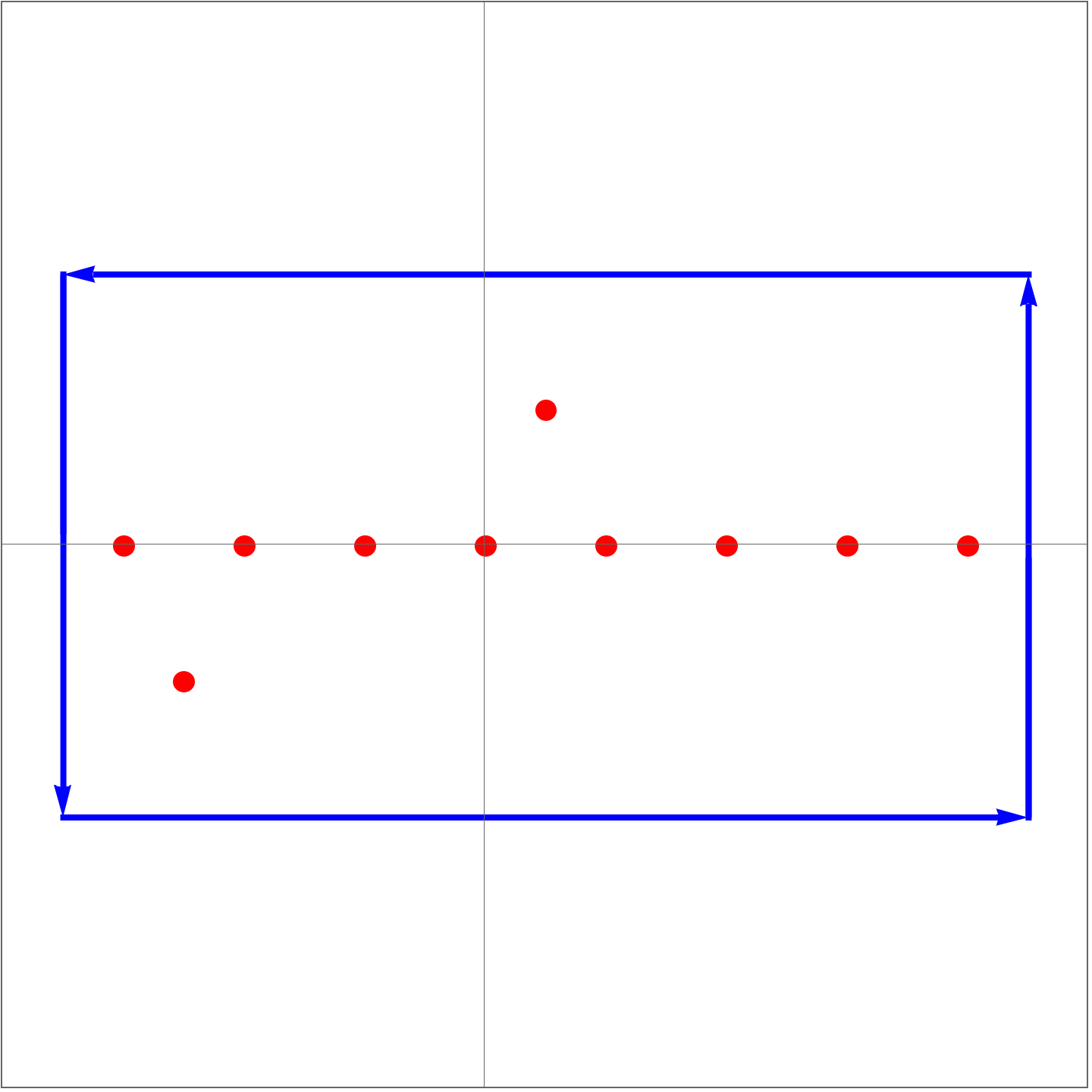
fig. 1. Directed distance from origin to line.
The geometry of the problem is illustrated in fig. 1.
Observe that all the calculation above was superfluous, as observation of the geometry shows that we just wanted the rejection of \( \mathbf{\hat{d}} \) (green) from \( \Bp \) (blue), and could have stated the result directly.
Distance between two lines.
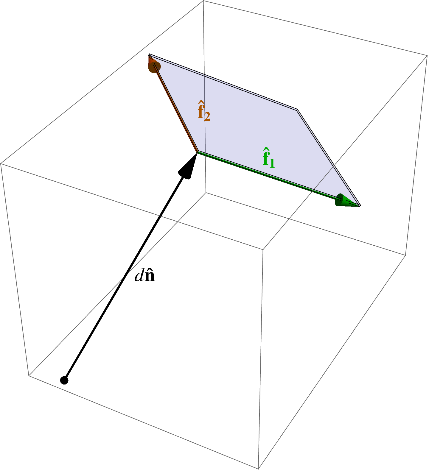
Suppose that we have two lines, specified with a point and direction vector for each line, as illustrated in fig. 2
\begin{equation}\label{eqn:shortestDistanceBetweenLines:20}
\begin{aligned}
L_1&: \Bx(r) = \Bp_1 + r \mathbf{\hat{d}}_1 \\
L_2&: \Bx(s) = \Bp_2 + s \mathbf{\hat{d}}_2 \\
\end{aligned}
\end{equation}

fig. 2. Two lines, not intersecting.
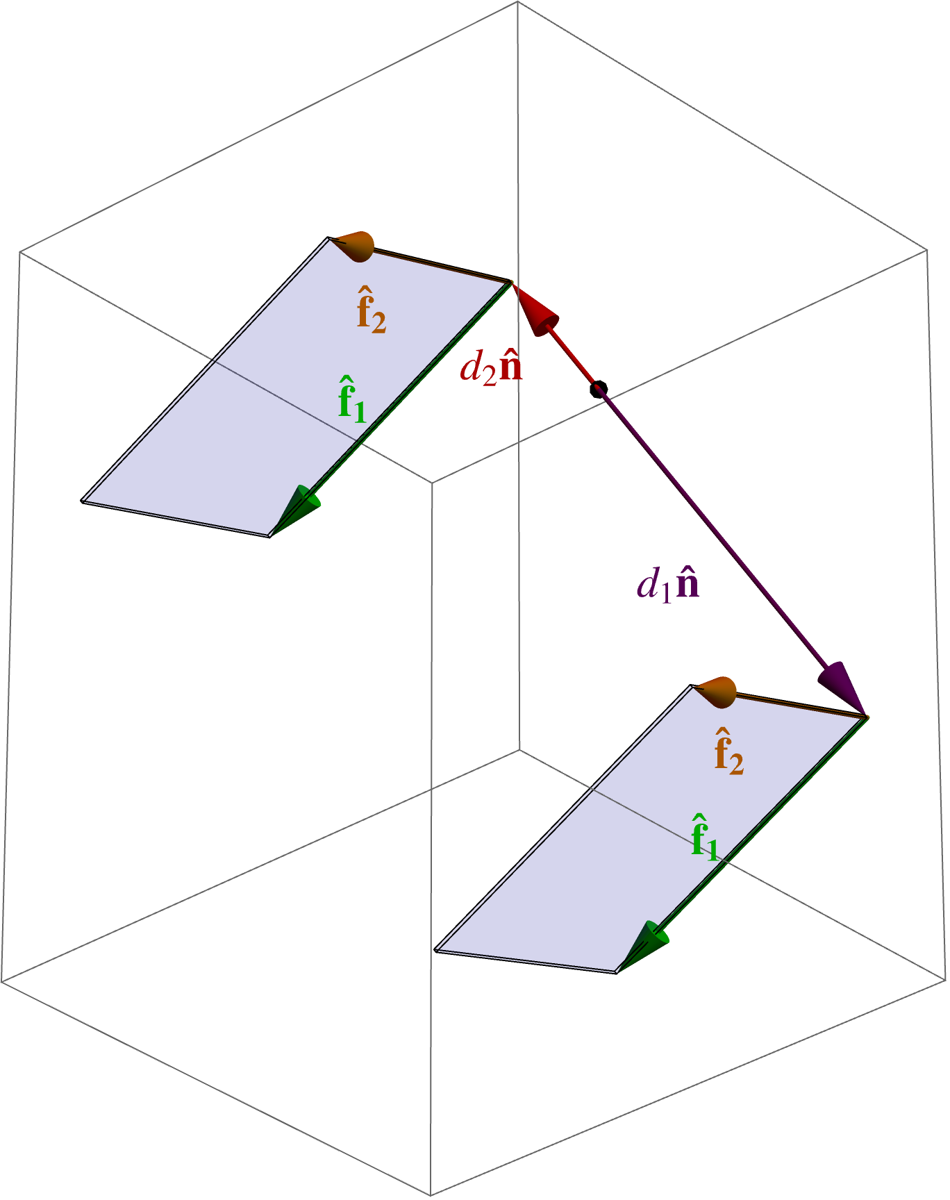
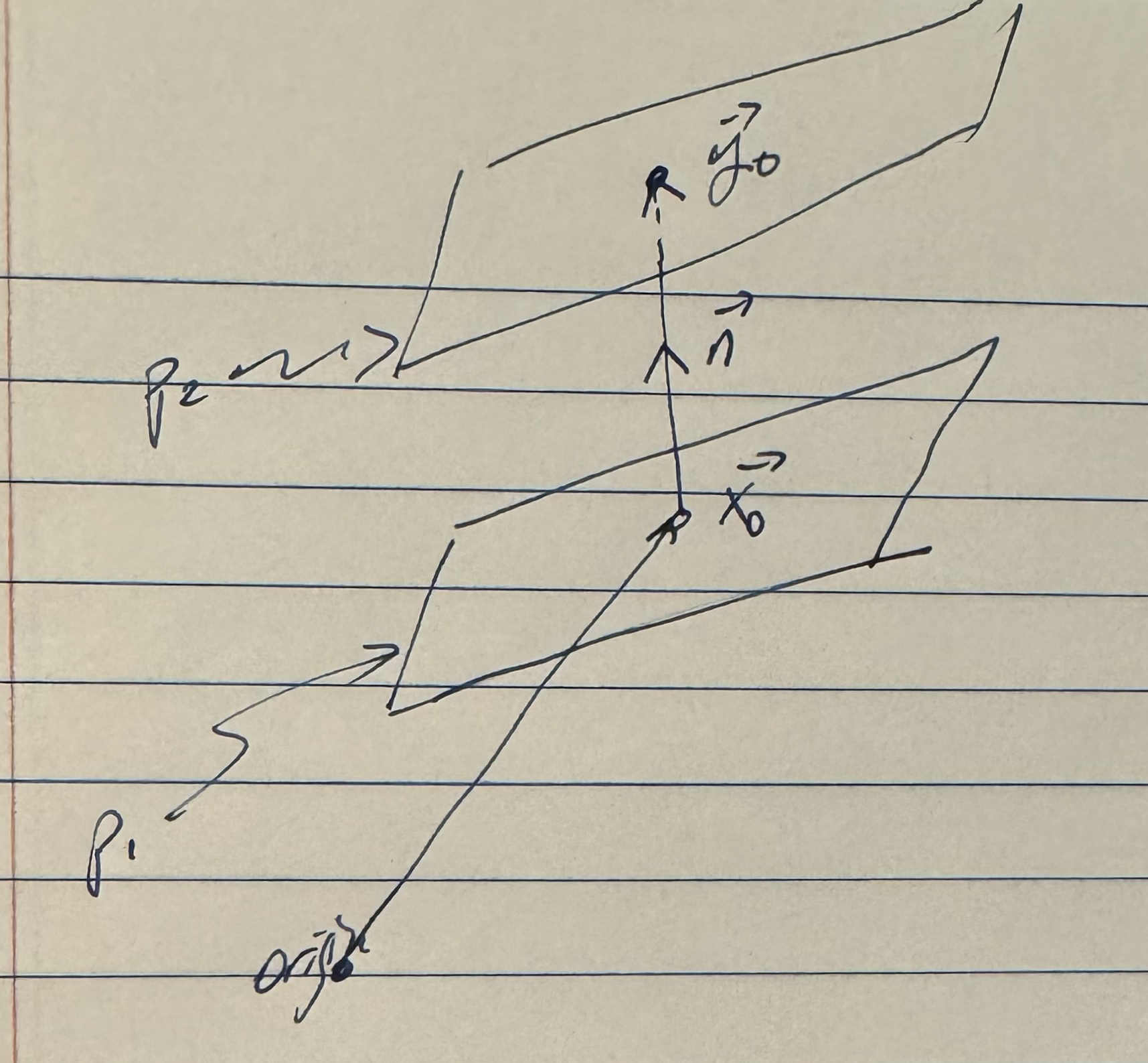
The geometry of the problem becomes more clear if we augment this figure, adding a line with the direction \( \mathbf{\hat{d}}_2 \) to \( L_1 \), and adding a line with the direction \( \mathbf{\hat{d}}_1 \) to \( L_2 \), as illustrated in fig. 3, and then visually extending each of those lines to planes that pass through the respective points. We can now rotate our viewpoint so that we look at those planes on edge, which shows that the problem to solve is really just the distance between two parallel planes.

fig 3a. Augmenting the lines with alternate direction vectors to form planes.

fig 3b. Rotation to view planes edge on.
The equations of these planes are just
\begin{equation}\label{eqn:shortestDistanceBetweenLines:160}
\begin{aligned}
P_1&: \Bx(r, s) = \Bp_1 + r \mathbf{\hat{d}}_1 + s \mathbf{\hat{d}}_2 \\
P_2&: \Bx(t, u) = \Bp_2 + t \mathbf{\hat{d}}_2 + u \mathbf{\hat{d}}_1,
\end{aligned}
\end{equation}
or with
\begin{equation}\label{eqn:shortestDistanceBetweenLines:180}
\mathbf{\hat{n}} = \frac{\mathbf{\hat{d}}_1 \cross \mathbf{\hat{d}}_2}{\Norm{\mathbf{\hat{d}}_1 \cross \mathbf{\hat{d}}_2}},
\end{equation}
the normal form for these planes are
\begin{equation}\label{eqn:shortestDistanceBetweenLines:200}
\begin{aligned}
P_1&: \Bx \cdot \mathbf{\hat{n}} = \Bp_1 \cdot \mathbf{\hat{n}} \\
P_2&: \Bx \cdot \mathbf{\hat{n}} = \Bp_2 \cdot \mathbf{\hat{n}}.
\end{aligned}
\end{equation}
Now we can state the distance between the planes trivially, using the results from our previous posts, finding
\begin{equation}\label{eqn:shortestDistanceBetweenLines:220}
d = \Abs{ \Bp_2 \cdot \mathbf{\hat{n}} – \Bp_1 \cdot \mathbf{\hat{n}} },
\end{equation}
or, encoding the triple product in it’s determinant form, the shortest distance between the lines (up to a sign), is
\begin{equation}\label{eqn:shortestDistanceBetweenLines:240}
\boxed{
d = \frac{
\begin{vmatrix}
\Bp_2 – \Bp_1 & \mathbf{\hat{d}}_1 & \mathbf{\hat{d}}_2
\end{vmatrix}
}{
\Norm{ \mathbf{\hat{d}}_1 \cross \mathbf{\hat{d}}_2 }
}.
}
\end{equation}
As a minimization problem.
Trying this as a minimization problem is actually kind of fun, albeit messy. Doing that calculation will give us the directed shortest distance between the lines.
We can form any number of vectors \( \Bm \) connecting the two lines
\begin{equation}\label{eqn:shortestDistanceBetweenLines:260}
\Bp_1 + s \mathbf{\hat{d}}_1 + \Bm = \Bp_2 + t \mathbf{\hat{d}}_2,
\end{equation}
or, with \( \Delta = \Bp_2 – \Bp_1 \), that directed distance is
\begin{equation}\label{eqn:shortestDistanceBetweenLines:280}
\Bm = \Delta + t \mathbf{\hat{d}}_2 – s \mathbf{\hat{d}}_1.
\end{equation}
We seek to minimize the squared length of this vector
\begin{equation}\label{eqn:shortestDistanceBetweenLines:300}
D = \Norm{\Bm}^2 = \Delta^2 + \lr{ t \mathbf{\hat{d}}_2 – s \mathbf{\hat{d}}_1 }^2 + 2 \Delta \cdot \lr{ t \mathbf{\hat{d}}_2 – s \mathbf{\hat{d}}_1 }.
\end{equation}
The minimization constraints are
\begin{equation}\label{eqn:shortestDistanceBetweenLines:320}
\begin{aligned}
0 &= \PD{s}{D} = 2 \lr{ t \mathbf{\hat{d}}_2 – s \mathbf{\hat{d}}_1 } \cdot \lr{ -\mathbf{\hat{d}}_1 } + 2 \Delta \cdot \lr{ – \mathbf{\hat{d}}_1 } \\
0 &= \PD{t}{D} = 2 \lr{ t \mathbf{\hat{d}}_2 – s \mathbf{\hat{d}}_1 } \cdot \lr{ \mathbf{\hat{d}}_2 } + 2 \Delta \cdot \lr{ \mathbf{\hat{d}}_2 }.
\end{aligned}
\end{equation}
With \( \alpha = \mathbf{\hat{d}}_1 \cdot \mathbf{\hat{d}}_2 \), our solution for \( s, t \) is
\begin{equation}\label{eqn:shortestDistanceBetweenLines:340}
\begin{bmatrix}
s \\
t
\end{bmatrix}
=
{
\begin{bmatrix}
1 & -\alpha \\
-\alpha & 1
\end{bmatrix}
}^{-1}
\begin{bmatrix}
\Delta \cdot \mathbf{\hat{d}}_1 \\
-\Delta \cdot \mathbf{\hat{d}}_2 \\
\end{bmatrix},
\end{equation}
so
\begin{equation}\label{eqn:shortestDistanceBetweenLines:360}
\begin{aligned}
t \mathbf{\hat{d}}_2 – s \mathbf{\hat{d}}_1
&=
\begin{bmatrix}
-\mathbf{\hat{d}}_1 & \mathbf{\hat{d}}_2
\end{bmatrix}
\begin{bmatrix}
s \\
t
\end{bmatrix} \\
&=
\inv{1 – \alpha^2}
\begin{bmatrix}
-\mathbf{\hat{d}}_1 & \mathbf{\hat{d}}_2
\end{bmatrix}
\begin{bmatrix}
1 & \alpha \\
\alpha & 1
\end{bmatrix}
\begin{bmatrix}
\Delta \cdot \mathbf{\hat{d}}_1 \\
-\Delta \cdot \mathbf{\hat{d}}_2 \\
\end{bmatrix} \\
&=
\inv{1 – \alpha^2}
\begin{bmatrix}
-\mathbf{\hat{d}}_1 & \mathbf{\hat{d}}_2
\end{bmatrix}
\begin{bmatrix}
\Delta \cdot \mathbf{\hat{d}}_1 – \alpha \Delta \cdot \mathbf{\hat{d}}_2 \\
\alpha \Delta \cdot \mathbf{\hat{d}}_1 -\Delta \cdot \mathbf{\hat{d}}_2 \\
\end{bmatrix} \\
&=
\inv{1 – \alpha^2}
\lr{
-\lr{ \Delta \cdot \mathbf{\hat{d}}_1} \mathbf{\hat{d}}_1 + \alpha \lr{ \Delta \cdot \mathbf{\hat{d}}_2} \mathbf{\hat{d}}_1
+
\alpha \lr{ \Delta \cdot \mathbf{\hat{d}}_1} \mathbf{\hat{d}}_2 – \lr{ \Delta \cdot \mathbf{\hat{d}}_2} \mathbf{\hat{d}}_2
} \\
&=
\inv{1 – \alpha^2}
\lr{
\lr{ \Delta \cdot \mathbf{\hat{d}}_1} \lr{
-\mathbf{\hat{d}}_1 + \alpha \mathbf{\hat{d}}_2
}
+
\lr{ \Delta \cdot \mathbf{\hat{d}}_2} \lr{
-\mathbf{\hat{d}}_2 + \alpha \mathbf{\hat{d}}_1
}
}.
\end{aligned}
\end{equation}
This might look a bit hopeless to simplify, but note that
\begin{equation}\label{eqn:shortestDistanceBetweenLines:380}
\begin{aligned}
\lr{ \mathbf{\hat{d}}_1 \wedge \mathbf{\hat{d}}_2}^2
&=
\lr{ \mathbf{\hat{d}}_1 \wedge \mathbf{\hat{d}}_2} \cdot \lr{ \mathbf{\hat{d}}_1 \wedge \mathbf{\hat{d}}_2} \\
&=
\mathbf{\hat{d}}_1 \cdot \lr{ \mathbf{\hat{d}}_2 \cdot \lr{ \mathbf{\hat{d}}_1 \wedge \mathbf{\hat{d}}_2} } \\
&=
\mathbf{\hat{d}}_1 \cdot \lr{ \alpha \mathbf{\hat{d}}_2 – \mathbf{\hat{d}}_1 } \\
&=
\alpha^2 – 1,
\end{aligned}
\end{equation}
and
\begin{equation}\label{eqn:shortestDistanceBetweenLines:400}
\begin{aligned}
\mathbf{\hat{d}}_2 \cdot \lr{ \mathbf{\hat{d}}_1 \wedge \mathbf{\hat{d}}_2} &= \alpha \mathbf{\hat{d}}_2 – \mathbf{\hat{d}}_1 \\
-\mathbf{\hat{d}}_1 \cdot \lr{ \mathbf{\hat{d}}_1 \wedge \mathbf{\hat{d}}_2} &= -\mathbf{\hat{d}}_2 + \alpha \mathbf{\hat{d}}_1.
\end{aligned}
\end{equation}
Let’s write \( B = \mathbf{\hat{d}}_1 \wedge \mathbf{\hat{d}}_2 \), and plug in our bivector expressions
\begin{equation}\label{eqn:shortestDistanceBetweenLines:420}
\begin{aligned}
t \mathbf{\hat{d}}_2 – s \mathbf{\hat{d}}_1
&=
-\inv{B^2}
\lr{
\lr{ \Delta \cdot \mathbf{\hat{d}}_1} \mathbf{\hat{d}}_2 \cdot B
-\lr{ \Delta \cdot \mathbf{\hat{d}}_2} \mathbf{\hat{d}}_1 \cdot B
} \\
&=
-\inv{B^2}
\lr{
\lr{ \Delta \cdot \mathbf{\hat{d}}_1} \mathbf{\hat{d}}_2
-\lr{ \Delta \cdot \mathbf{\hat{d}}_2} \mathbf{\hat{d}}_1
}
\cdot B \\
&=
-\inv{B^2}
\lr{
\Delta \cdot \lr{ \mathbf{\hat{d}}_1 \wedge \mathbf{\hat{d}}_2}
}
\cdot B \\
&=
-\inv{B^2} \lr{ \Delta \cdot B } \cdot B \\
&=
-\inv{B^2} \gpgradeone{ \lr{ \Delta \cdot B } B } \\
&=
-\inv{B^2} \gpgradeone{ \lr{ \Delta B – \Delta \wedge B } B } \\
&=
-\Delta + \inv{B^2} \lr{ \Delta \wedge B } \cdot B.
\end{aligned}
\end{equation}
The minimum directed distance between the lines is now reduced to just
\begin{equation}\label{eqn:shortestDistanceBetweenLines:440}
\begin{aligned}
\Bm
&= \Delta + t \mathbf{\hat{d}}_2 – s \mathbf{\hat{d}}_1 \\
&= \lr{ \Delta \wedge B } \inv{B}.
\end{aligned}
\end{equation}
Again, had we used the geometry effectively, illustrated in fig. 4, we could have skipped directly to this result. This is the rejection of the plane \( B \) from \( \Delta \), that is, rejection of both \( \mathbf{\hat{d}}_1, \mathbf{\hat{d}}_2 \) from the difference \( \Bp_2 – \Bp_1 \), leaving just the perpendicular shortest connector between the lines.

fig. 4. Projection onto the normal to the parallel planes.
We can also conceptualize this as computing the trivector volume (parallelepiped with edges \( \Bp_2 – \Bp_1, \mathbf{\hat{d}}_1, \mathbf{\hat{d}}_2 \)), and then dividing out the bivector (parallelogram with edges \(\mathbf{\hat{d}}_1, \mathbf{\hat{d}}_2 \)), to find the vector (height) of the parallelepiped.
Observe that rejecting from the plane, is equivalent to projecting onto the normal, so for \(\mathbb{R}^3\) we may translate this to conventional vector algebra, as a projection
\begin{equation}\label{eqn:shortestDistanceBetweenLines:500}
\Bm = \lr{\Delta \cdot \mathbf{\hat{n}}} \mathbf{\hat{n}},
\end{equation}
where \( \mathbf{\hat{n}} = \lr{ \mathbf{\hat{d}}_1 \cross \mathbf{\hat{d}}_2 }/\Norm{\mathbf{\hat{d}}_1 \cross \mathbf{\hat{d}}_2 } \).
If we want the magnitude of this vector, it’s just
\begin{equation}\label{eqn:shortestDistanceBetweenLines:480}
\begin{aligned}
\Norm{\Bm}^2
&=
\inv{B^4} \lr{ \lr{ \Delta \wedge B } B } \lr{ B \lr{ B \wedge \Delta } } \\
&=
\inv{B^2} \lr{ \Delta \wedge B }^2,
\end{aligned}
\end{equation}
or
\begin{equation}\label{eqn:shortestDistanceBetweenLines:460}
\boxed{
\Norm{\Bm} = \frac{ \Norm{ \lr{\Bp_2 – \Bp_1} \wedge \mathbf{\hat{d}}_1 \wedge \mathbf{\hat{d}}_2 } }{ \Norm{\mathbf{\hat{d}}_1 \wedge \mathbf{\hat{d}}_2} },
}
\end{equation}
which, for \(\mathbb{R}^3\), is equivalent to the triple product result we found above.
Like this:
Like Loading...