phy1520

Can anticommuting operators have a simulaneous eigenket?

September 28, 2015 phy1520 , ,

[Click here for a PDF of this post with nicer formatting]

Question: Can anticommuting operators have a simulaneous eigenket? ([1] pr. 1.16)

Two Hermitian operators anticommute

\begin{equation}\label{eqn:anticommutingOperatorWithSimulaneousEigenket:20}
\symmetric{A}{B} = A B + B A = 0.
\end{equation}

Is it possible to have a simultaneous eigenket of \( A \) and \( B \)? Prove or illustrate your assertion.

Answer

Suppose that such a simultaneous non-zero eigenket \( \ket{\alpha} \) exists, then

\begin{equation}\label{eqn:anticommutingOperatorWithSimulaneousEigenket:40}
A \ket{\alpha} = a \ket{\alpha},
\end{equation}

and

\begin{equation}\label{eqn:anticommutingOperatorWithSimulaneousEigenket:60}
B \ket{\alpha} = b \ket{\alpha}
\end{equation}

This gives

\begin{equation}\label{eqn:anticommutingOperatorWithSimulaneousEigenket:80}
\lr{ A B + B A } \ket{\alpha}
=
\lr{A b + B a} \ket{\alpha}
= 2 a b \ket{\alpha}.
\end{equation}

If this is zero, one of the operators must have a zero eigenvalue. Knowing that we can construct an example of such operators. In matrix form, let

\begin{equation}\label{eqn:anticommutingOperatorWithSimulaneousEigenket:120}
A =
\begin{bmatrix}
1 & 0 & 0 \\
0 & -1 & 0 \\
0 & 0 & a \\
\end{bmatrix}
\end{equation}
\begin{equation}\label{eqn:anticommutingOperatorWithSimulaneousEigenket:140}
B =
\begin{bmatrix}
0 & 1 & 0 \\
1 & 0 & 0 \\
0 & 0 & b \\
\end{bmatrix}.
\end{equation}

These are both Hermitian, and anticommute provided at least one of \( a, b\) is zero. These have a common eigenket

\begin{equation}\label{eqn:anticommutingOperatorWithSimulaneousEigenket:160}
\ket{\alpha} =
\begin{bmatrix}
0 \\
0 \\
1
\end{bmatrix}.
\end{equation}

A zero eigenvalue of one of the commuting operators may not be a sufficient condition for such anticommutation.

References

[1] Jun John Sakurai and Jim J Napolitano. Modern quantum mechanics. Pearson Higher Ed, 2014.

Lagrangian for magnetic portion of Lorentz force

September 26, 2015 phy1520 , , , ,

[Click here for a PDF of this post with nicer formatting]

In [1] it is claimed in an Aharonov-Bohm discussion that a Lagrangian modification to include electromagnetism is

\begin{equation}\label{eqn:magneticLorentzForceLagrangian:20}
\LL \rightarrow \LL + \frac{e}{c} \Bv \cdot \BA.
\end{equation}

That can’t be the full Lagrangian since there is no \( \phi \) term, so what exactly do we get?

If you have somehow, like I did, forgot the exact form of the Euler-Lagrange equations (i.e. where do the dots go), then the derivation of those equations can come to your rescue. The starting point is the action

\begin{equation}\label{eqn:magneticLorentzForceLagrangian:40}
S = \int \LL(x, \xdot, t) dt,
\end{equation}

where the end points of the integral are fixed, and we assume we have no variation at the end points. The variational calculation is

\begin{equation}\label{eqn:magneticLorentzForceLagrangian:60}
\begin{aligned}
\delta S
&= \int \delta \LL(x, \xdot, t) dt \\
&= \int \lr{ \PD{x}{\LL} \delta x + \PD{\xdot}{\LL} \delta \xdot } dt \\
&= \int \lr{ \PD{x}{\LL} \delta x + \PD{\xdot}{\LL} \delta \ddt{x} } dt \\
&= \int \lr{ \PD{x}{\LL} – \ddt{}\lr{\PD{\xdot}{\LL}} } \delta x dt
+ \delta x \PD{\xdot}{\LL}.
\end{aligned}
\end{equation}

The boundary term is killed after evaluation at the end points where the variation is zero. For the result to hold for all variations \( \delta x \), we must have

\begin{equation}\label{eqn:magneticLorentzForceLagrangian:80}
\boxed{
\PD{x}{\LL} = \ddt{}\lr{\PD{\xdot}{\LL}}.
}
\end{equation}

Now lets apply this to the Lagrangian at hand. For the position derivative we have

\begin{equation}\label{eqn:magneticLorentzForceLagrangian:100}
\PD{x_i}{\LL}
=
\frac{e}{c} v_j \PD{x_i}{A_j}.
\end{equation}

For the canonical momentum term, assuming \( \BA = \BA(\Bx) \) we have

\begin{equation}\label{eqn:magneticLorentzForceLagrangian:120}
\begin{aligned}
\ddt{} \PD{\xdot_i}{\LL}
&=
\ddt{}
\lr{ m \xdot_i
+
\frac{e}{c} A_i
} \\
&=
m \ddot{x}_i
+
\frac{e}{c}
\ddt{A_i} \\
&=
m \ddot{x}_i
+
\frac{e}{c}
\PD{x_j}{A_i} \frac{dx_j}{dt}.
\end{aligned}
\end{equation}

Assembling the results, we’ve got

\begin{equation}\label{eqn:magneticLorentzForceLagrangian:140}
\begin{aligned}
0
&=
\ddt{} \PD{\xdot_i}{\LL}

\PD{x_i}{\LL} \\
&=
m \ddot{x}_i
+
\frac{e}{c}
\PD{x_j}{A_i} \frac{dx_j}{dt}

\frac{e}{c} v_j \PD{x_i}{A_j},
\end{aligned}
\end{equation}

or
\begin{equation}\label{eqn:magneticLorentzForceLagrangian:160}
\begin{aligned}
m \ddot{x}_i
&=
\frac{e}{c} v_j \PD{x_i}{A_j}

\frac{e}{c}
\PD{x_j}{A_i} v_j \\
&=
\frac{e}{c} v_j
\lr{
\PD{x_i}{A_j}

\PD{x_j}{A_i}
} \\
&=
\frac{e}{c} v_j B_k \epsilon_{i j k}.
\end{aligned}
\end{equation}

In vector form that is

\begin{equation}\label{eqn:magneticLorentzForceLagrangian:180}
m \ddot{\Bx}
=
\frac{e}{c} \Bv \cross \BB.
\end{equation}

So, we get the magnetic term of the Lorentz force. Also note that this shows the Lagrangian (and the end result), was not in SI units. The \( 1/c \) term would have to be dropped for SI.

References

[1] Jun John Sakurai and Jim J Napolitano. Modern quantum mechanics. Pearson Higher Ed, 2014.

PHY1520H Graduate Quantum Mechanics. Lecture 3: Density matrix (cont.). Taught by Prof. Arun Paramekanti

September 24, 2015 phy1520 , , , , , , , , ,

[Click here for a PDF of this post with nicer formatting]

Disclaimer

Peeter’s lecture notes from class. These may be incoherent and rough.

These are notes for the UofT course PHY1520, Graduate Quantum Mechanics, taught by Prof. Paramekanti, covering [1] chap. 3 content.

Density matrix (cont.)

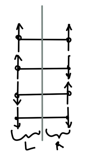
An example of a partitioned system with four total states (two spin 1/2 particles) is sketched in fig. 1.
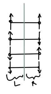
fig. 1.  Two spins

fig. 1. Two spins

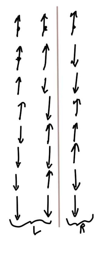
An example of a partitioned system with eight total states (three spin 1/2 particles) is sketched in fig. 2.
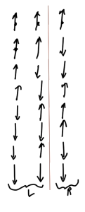
fig. 2.  Three spins

fig. 2. Three spins

The density matrix

\begin{equation}\label{eqn:qmLecture3:20}
\hat{\rho} = \ket{\Psi}\bra{\Psi}
\end{equation}

is clearly an operator as can be seen by applying it to a state

\begin{equation}\label{eqn:qmLecture3:40}
\hat{\rho} \ket{\phi} = \ket{\Psi} \lr{ \braket{ \Psi }{\phi} }.
\end{equation}

The quantity in braces is just a complex number.

After expanding the pure state \( \ket{\Psi} \) in terms of basis states for each of the two partitions

\begin{equation}\label{eqn:qmLecture3:60}
\ket{\Psi}
= \sum_{m,n} C_{m, n} \ket{m}_{\textrm{L}} \ket{n}_{\textrm{R}},
\end{equation}

With \( \textrm{L} \) and \( \textrm{R} \) implied for \( \ket{m}, \ket{n} \) indexed states respectively, this can be written

\begin{equation}\label{eqn:qmLecture3:460}
\ket{\Psi}
= \sum_{m,n} C_{m, n} \ket{m} \ket{n}.
\end{equation}

The density operator is

\begin{equation}\label{eqn:qmLecture3:80}
\hat{\rho} =
\sum_{m,n}
C_{m, n}
C_{m’, n’}^\conj
\ket{m} \ket{n}
\sum_{m’,n’}
\bra{m’} \bra{n’}.
\end{equation}

Suppose we trace over the right partition of the state space, defining such a trace as the reduced density operator \( \hat{\rho}_{\textrm{red}} \)

\begin{equation}\label{eqn:qmLecture3:100}
\begin{aligned}
\hat{\rho}_{\textrm{red}}
&\equiv
\textrm{Tr}_{\textrm{R}}(\hat{\rho}) \\
&= \sum_{\tilde{n}} \bra{\tilde{n}} \hat{\rho} \ket{ \tilde{n}} \\
&= \sum_{\tilde{n}}
\bra{\tilde{n} }
\lr{
\sum_{m,n}
C_{m, n}
\ket{m} \ket{n}
}
\lr{
\sum_{m’,n’}
C_{m’, n’}^\conj
\bra{m’} \bra{n’}
}
\ket{ \tilde{n} } \\
&=
\sum_{\tilde{n}}
\sum_{m,n}
\sum_{m’,n’}
C_{m, n}
C_{m’, n’}^\conj
\ket{m} \delta_{\tilde{n} n}
\bra{m’ }
\delta_{ \tilde{n} n’ } \\
&=
\sum_{\tilde{n}, m, m’}
C_{m, \tilde{n}}
C_{m’, \tilde{n}}^\conj
\ket{m} \bra{m’ }
\end{aligned}
\end{equation}

Computing the matrix element of \( \hat{\rho}_{\textrm{red}} \), we have

\begin{equation}\label{eqn:qmLecture3:120}
\begin{aligned}
\bra{\tilde{m}} \hat{\rho}_{\textrm{red}} \ket{\tilde{m}}
&=
\sum_{m, m’, \tilde{n}} C_{m, \tilde{n}} C_{m’, \tilde{n}}^\conj \braket{ \tilde{m}}{m} \braket{m’}{\tilde{m}} \\
&=
\sum_{\tilde{n}} \Abs{C_{\tilde{m}, \tilde{n}} }^2.
\end{aligned}
\end{equation}

This is the probability that the left partition is in state \( \tilde{m} \).

Average of an observable

Suppose we have two spin half particles. For such a system the total magnetization is

\begin{equation}\label{eqn:qmLecture3:140}
S_{\textrm{Total}} =
S_1^z
+
S_1^z,
\end{equation}

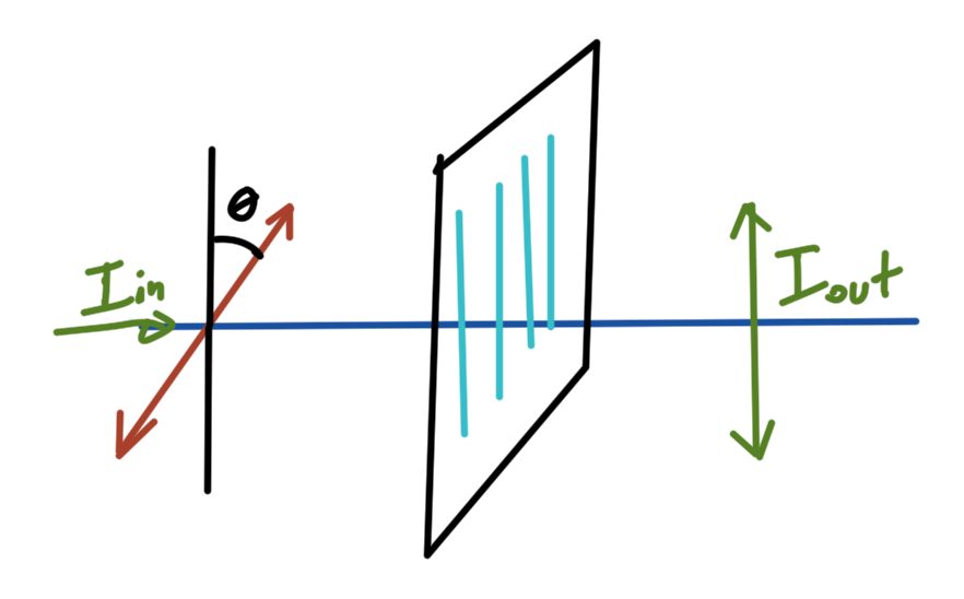
as sketched in fig. 3.

fig. 3.  Magnetic moments from two spins.

fig. 3. Magnetic moments from two spins.

The average of some observable is

\begin{equation}\label{eqn:qmLecture3:160}
\expectation{\hatA}
= \sum_{m, n, m’, n’} C_{m, n}^\conj C_{m’, n’}
\bra{m}\bra{n} \hatA \ket{n’} \ket{m’}.
\end{equation}

Consider the trace of the density operator observable product

\begin{equation}\label{eqn:qmLecture3:180}
\textrm{Tr}( \hat{\rho} \hatA )
= \sum_{m, n} \braket{m n}{\Psi} \bra{\Psi} \hatA \ket{m, n}.
\end{equation}

Let

\begin{equation}\label{eqn:qmLecture3:200}
\ket{\Psi} = \sum_{m, n} C_{m n} \ket{m, n},
\end{equation}

so that

\begin{equation}\label{eqn:qmLecture3:220}
\begin{aligned}
\textrm{Tr}( \hat{\rho} \hatA )
&= \sum_{m, n, m’, n’, m”, n”} C_{m’, n’} C_{m”, n”}^\conj
\braket{m n}{m’, n’} \bra{m”, n”} \hatA \ket{m, n} \\
&= \sum_{m, n, m”, n”} C_{m, n} C_{m”, n”}^\conj
\bra{m”, n”} \hatA \ket{m, n}.
\end{aligned}
\end{equation}

This is just

\begin{equation}\label{eqn:qmLecture3:240}
\boxed{
\bra{\Psi} \hatA \ket{\Psi} = \textrm{Tr}( \hat{\rho} \hatA ).
}
\end{equation}

Left observables

Consider

\begin{equation}\label{eqn:qmLecture3:260}
\begin{aligned}
\bra{\Psi} \hatA_{\textrm{L}} \ket{\Psi}
&= \textrm{Tr}(\hat{\rho} \hatA_{\textrm{L}}) \\
&=
\textrm{Tr}_{\textrm{L}}
\textrm{Tr}_{\textrm{R}}
(\hat{\rho} \hatA_{\textrm{L}}) \\
&=
\textrm{Tr}_{\textrm{L}}
\lr{
\lr{
\textrm{Tr}_{\textrm{R}} \hat{\rho}
}
\hatA_{\textrm{L}})
} \\
&=
\textrm{Tr}_{\textrm{L}}
\lr{
\hat{\rho}_{\textrm{red}}
\hatA_{\textrm{L}})
}.
\end{aligned}
\end{equation}

We see

\begin{equation}\label{eqn:qmLecture3:280}
\bra{\Psi} \hatA_{\textrm{L}} \ket{\Psi}
=
\textrm{Tr}_{\textrm{L}} \lr{ \hat{\rho}_{\textrm{red}, \textrm{L}} \hatA_{\textrm{L}} }.
\end{equation}

We find that we don’t need to know the state of the complete system to answer questions about portions of the system, but instead just need \( \hat{\rho} \), a “probability operator” that provides all the required information about the partitioning of the system.

Pure states vs. mixed states

For pure states we can assign a state vector and talk about reduced scenarios. For mixed states we must work with reduced density matrix.

Example: Two particle spin half pure states

Consider

\begin{equation}\label{eqn:qmLecture3:300}
\ket{\psi_1} = \inv{\sqrt{2}} \lr{ \ket{ \uparrow \downarrow } – \ket{ \downarrow \uparrow } }
\end{equation}

\begin{equation}\label{eqn:qmLecture3:320}
\ket{\psi_2} = \inv{\sqrt{2}} \lr{ \ket{ \uparrow \downarrow } + \ket{ \uparrow \uparrow } }.
\end{equation}

For the first pure state the density operator is
\begin{equation}\label{eqn:qmLecture3:360}
\hat{\rho} = \inv{2}
\lr{ \ket{ \uparrow \downarrow } – \ket{ \downarrow \uparrow } }
\lr{ \bra{ \uparrow \downarrow } – \bra{ \downarrow \uparrow } }
\end{equation}

What are the reduced density matrices?

\begin{equation}\label{eqn:qmLecture3:340}
\begin{aligned}
\hat{\rho}_{\textrm{L}}
&= \textrm{Tr}_{\textrm{R}} \lr{ \hat{\rho} } \\
&=
\inv{2} (-1)(-1) \ket{\downarrow}\bra{\downarrow}
+\inv{2} (+1)(+1) \ket{\uparrow}\bra{\uparrow},
\end{aligned}
\end{equation}

so the matrix representation of this reduced density operator is

\begin{equation}\label{eqn:qmLecture3:380}
\hat{\rho}_{\textrm{L}}
=
\inv{2}
\begin{bmatrix}
1 & 0 \\
0 & 1
\end{bmatrix}.
\end{equation}

For the second pure state the density operator is
\begin{equation}\label{eqn:qmLecture3:400}
\hat{\rho} = \inv{2}
\lr{ \ket{ \uparrow \downarrow } + \ket{ \uparrow \uparrow } }
\lr{ \bra{ \uparrow \downarrow } + \bra{ \uparrow \uparrow } }.
\end{equation}

This has a reduced density matrice

\begin{equation}\label{eqn:qmLecture3:420}
\begin{aligned}
\hat{\rho}_{\textrm{L}}
&= \textrm{Tr}_{\textrm{R}} \lr{ \hat{\rho} } \\
&=
\inv{2} \ket{\uparrow}\bra{\uparrow}
+\inv{2} \ket{\uparrow}\bra{\uparrow} \\
&=
\ket{\uparrow}\bra{\uparrow} .
\end{aligned}
\end{equation}

This has a matrix representation

\begin{equation}\label{eqn:qmLecture3:440}
\hat{\rho}_{\textrm{L}}
=
\begin{bmatrix}
1 & 0 \\
0 & 0
\end{bmatrix}.
\end{equation}

In this second example, we have more information about the left partition. That will be seen as a zero entanglement entropy in the problem set. In contrast we have less information about the first state, and will find a non-zero positive entanglement entropy in that case.

References

[1] Jun John Sakurai and Jim J Napolitano. Modern quantum mechanics. Pearson Higher Ed, 2014.

Constant magnetic solenoid field

September 24, 2015 phy1520 , , , , ,

[Click here for a PDF of this post with nicer formatting]

In [2] the following vector potential

\begin{equation}\label{eqn:solenoidConstantField:20}
\BA = \frac{B \rho_a^2}{2 \rho} \phicap,
\end{equation}

is introduced in a discussion on the Aharonov-Bohm effect, for configurations where the interior field of a solenoid is either a constant \( \BB \) or zero.

I wasn’t able to make sense of this since the field I was calculating was zero for all \( \rho \ne 0 \)

\begin{equation}\label{eqn:solenoidConstantField:40}
\begin{aligned}
\BB
&= \spacegrad \cross \BA \\
&= \lr{ \rhocap \partial_\rho + \zcap \partial_z + \frac{\phicap}{\rho}
\partial_\phi } \cross \frac{B \rho_a^2}{2 \rho} \phicap \\
&= \lr{ \rhocap \partial_\rho + \frac{\phicap}{\rho} \partial_\phi } \cross
\frac{B \rho_a^2}{2 \rho} \phicap \\
&=
\frac{B \rho_a^2}{2}
\rhocap \cross \phicap \partial_\rho \lr{ \inv{\rho} }
+
\frac{B \rho_a^2}{2 \rho}
\frac{\phicap}{\rho} \cross \partial_\phi \phicap \\
&=
\frac{B \rho_a^2}{2 \rho^2} \lr{ -\zcap + \phicap \cross \partial_\phi \phicap}.
\end{aligned}
\end{equation}

Note that the \( \rho \) partial requires that \( \rho \ne 0 \). To expand the cross product in the second term let \( j = \Be_1 \Be_2 \), and expand using a Geometric Algebra representation of the unit vector

\begin{equation}\label{eqn:solenoidConstantField:60}
\begin{aligned}
\phicap \cross \partial_\phi \phicap
&=
\Be_2 e^{j \phi} \cross \lr{ \Be_2 \Be_1 \Be_2 e^{j \phi} } \\
&=
– \Be_1 \Be_2 \Be_3
\gpgradetwo{
\Be_2 e^{j \phi} (-\Be_1) e^{j \phi}
} \\
&=
\Be_1 \Be_2 \Be_3 \Be_2 \Be_1 \\
&= \Be_3 \\
&= \zcap.
\end{aligned}
\end{equation}

So, provided \( \rho \ne 0 \), \( \BB = 0 \).

The errata [1] provides the clarification, showing that a \( \rho > \rho_a \) constraint is required for this potential to produce the desired results. Continuity at \( \rho = \rho_a \) means that in the interior (or at least on the boundary) we must have one of

\begin{equation}\label{eqn:solenoidConstantField:80}
\BA = \frac{B \rho_a}{2} \phicap,
\end{equation}

or

\begin{equation}\label{eqn:solenoidConstantField:100}
\BA = \frac{B \rho}{2} \phicap.
\end{equation}

The first doesn’t work, but the second does

\begin{equation}\label{eqn:solenoidConstantField:120}
\begin{aligned}
\BB
&= \spacegrad \cross \BA \\
&= \lr{ \rhocap \partial_\rho + \zcap \partial_z + \frac{\phicap}{\rho}
\partial_\phi } \cross \frac{B \rho}{2 } \phicap \\
&=
\frac{B }{2 } \rhocap \cross \phicap
+
\frac{B \rho}{2 }
\frac{\phicap}{\rho} \cross \partial_\phi \phicap \\
&= B \zcap.
\end{aligned}
\end{equation}

So the vector potential that we want for a constant \( B \zcap \) field in the interior \( \rho < \rho_a \) of a cylindrical space, we need

\begin{equation}\label{eqn:solenoidConstantField:140}
\BA =
\left\{
\begin{array}{l l}
\frac{B \rho_a^2}{2 \rho} \phicap & \quad \mbox{if \( \rho \ge \rho_a \) } \\
\frac{B \rho}{2} \phicap & \quad \mbox{if \( \rho \le \rho_a \).}
\end{array}
\right.
\end{equation}

An example of the magnitude of potential is graphed in fig. 1.

solenoidPotentialFig1

fig. 1. Vector potential for constant field in cylindrical region.


References

[1] Jun John Sakurai and Jim J Napolitano. \emph{Errata: Typographical Errors, Mistakes, and Comments, Modern Quantum Mechanics, 2nd Edition}, 2013. URL http://www.rpi.edu/dept/phys/Courses/PHYS6520/Spring2015/ErrataMQM.pdf.

[2] Jun John Sakurai and Jim J Napolitano. Modern quantum mechanics. Pearson Higher Ed, 2014.

PHY1520H Graduate Quantum Mechanics. Lecture 2: Basic concepts, time evolution, and density operators. Taught by Prof. Arun Paramekanti

September 22, 2015 phy1520 , , ,

[Click here for a PDF of this post with nicer formatting]

Disclaimer

Peeter’s lecture notes from class. These may be incoherent and rough.

These are notes for the UofT course PHY1520, Graduate Quantum Mechanics, taught by Prof. Paramekanti, covering chap 1 (basic concepts),3 (density operator). content from [1].

Basic concepts

We’ve reviewed the basic concepts that we will encounter in Quantum Mechanics.

  1. Abstract state vector. \( \ket{ \psi} \)
  2. Basis states. \( \ket{ x } \)
  3. Observables, special Hermitian operators. We’ll only deal with linear observables.
  4. Measurement.

We can either express the wave functions \( \psi(x) = \braket{x}{\psi} \) in terms of a basis for the observable, or can express the observable in terms of the basis of the wave function (position or momentum for example).

We saw that the position space representation of a momentum operator (also an observable) was

\begin{equation}\label{eqn:lecture2:20}
\hat{p} \rightarrow -i \Hbar \PD{x}{}.
\end{equation}

In general we can find the matrix element representation of any operator by considering its representation in a given basis. For example, in a position basis, that would be

\begin{equation}\label{eqn:lecture2:40}
\bra{x’} \hat{A} \ket{x} \leftrightarrow A_{x x’}
\end{equation}

The Hermitian property of the observable means that \( A_{x x’} = A_{x’ x}^\conj \)

\begin{equation}\label{eqn:lecture2:60}
\int dx \bra{x’} \hat{A} \ket{x} \braket{x }{\psi} = \braket{x’}{\phi}
\leftrightarrow
A_{x’ x} \psi_x = \phi_{x’}.
\end{equation}

Example: Measurement example


polarizerMeasurementFig1

fig. 1. Polarizer apparatus

Consider a polarization apparatus as sketched in fig. 1, where the output is of the form \( I_{\textrm{out}} = I_{\textrm{in}} \cos^2 \theta \).

A general input state can be written in terms of each of the possible polarizations

\begin{equation}\label{eqn:lecture2:80}
\alpha \ket{ \updownarrow } + \beta \ket{ \leftrightarrow } \sim
\cos\theta \ket{ \updownarrow } + \sin\theta \ket{ \leftrightarrow }
\end{equation}

Here \( \abs{\alpha}^2 \) is the probability that the input state is in the upwards polarization state, and \( \abs{\beta}^2 \) is the probability that the input state is in the downwards polarization state.

The measurement of the polarization results in an output state that has a specific polarization. That measurement is said to collapse the wavefunction.

When attempting a measurement, looking for a specific value, effects the state of the system, and is call a strong or projective measurement. Such a measurement is

  • (i) Probabilistic.
  • (ii) Requires many measurements.

This measurement process results a determination of the eigenvalue of the operator. The eigenvalue production of measurement is why we demand that operators be Hermitian.

It is also possible to try to do a weaker (perturbative) measurement, where some information is extracted from the input state without completely altering it.

Time evolution

  1. Schrodinger picture.
    The time evolution process is governed by a Schrodinger equation of the following form\begin{equation}\label{eqn:lecture2:100}
    i \Hbar \PD{t}{} \ket{\Psi(t)} = \hat{H} \ket{\Psi(t)}.
    \end{equation}

    This Hamiltonian could be, for example,

    \begin{equation}\label{eqn:lecture2:120}
    \hat{H} = \frac{\hat{p}^2}{2m} + V(x),
    \end{equation}

    Such a representation of time evolution is expressed in terms of operators \( \hat{x}, \hat{p}, \hat{H}, \cdots \) that are independent of time.

  2. Heisenberg picture.Suppose we have a state \( \ket{\Psi(t)} \) and operate on this with an operator

    \begin{equation}\label{eqn:lecture2:140}
    \hat{A} \ket{\Psi(t)}.
    \end{equation}

    This will have time evolution of the form

    \begin{equation}\label{eqn:lecture2:160}
    \hat{A} e^{-i \hat{H} t/\Hbar} \ket{\Psi(0)},
    \end{equation}

    or in matrix element form

    \begin{equation}\label{eqn:lecture2:180}
    \bra{\phi(t)} \hat{A} \ket{\Psi(t)}
    =
    \bra{\phi(0)}
    e^{i \hat{H} t/\Hbar}
    \hat{A} e^{-i \hat{H} t/\Hbar} \ket{\Psi(0)}.
    \end{equation}

    We work with states that do not evolve in time \( \ket{\phi(0)}, \ket{\Psi(0)}, \cdots \), but operators do evolve in time according to

    \begin{equation}\label{eqn:lecture2:200}
    \hat{A}(t) =
    e^{i \hat{H} t/\Hbar}
    \hat{A} e^{-i \hat{H} t/\Hbar}.
    \end{equation}

Density operator

We can have situations where it is impossible to determine a single state that describes the system. For example, given the gas in the room that you are sitting in, there are things that we can measure, but it is impossible to describe the state that describes all the particles and also impossible to construct a Hamiltonian that governs all the interactions of those many many particles.

We need a probabilistic description to even describe such a complex system.

Suppose we have a complex system that can be partitioned into two subsets, left and right, as sketched in fig. 2.

fig. 2. System partitioned into separate set of states

fig. 2. System partitioned into separate set of states


If the states in each partition can be enumerated separately, we can write the state of the system as sums over the probability amplitudes that for the combined states.

\begin{equation}\label{eqn:lecture2:220}
\ket{\Psi}
=
\sum_{m, n} C_{m,n} \ket{m} \ket{n}
\end{equation}

Here \( C_{m, n} \) is the probability amplitude to find the state in the combined state \( \ket{m} \ket{n} \).

As an example of such a system, we could investigate a two particle configuration where spin up or spin down can be separately measured for each particle.

\begin{equation}\label{eqn:lecture2:240}
\ket{\psi} = \inv{\sqrt{2}} \lr{
\ket{\uparrow}\ket{\downarrow}
+
\ket{\downarrow}\ket{\rightarrow}
}
\end{equation}

Considering such a system we could ask questions such as

  • What is the probability that the left half is in state \( m \)? This would be\begin{equation}\label{eqn:lecture2:260}
    \sum_n \Abs{C_{m, n}}^2
    \end{equation}
  • Probability that the left half is in state \( m \), and the
    probability that the right half is in state \( n \)? That is\begin{equation}\label{eqn:lecture2:280}
    \Abs{C_{m, n}}^2
    \end{equation}

We define the density operator

\begin{equation}\label{eqn:lecture2:300}
\hat{\rho} = \ket{\Psi} \bra{\Psi}.
\end{equation}

This is idempotent

\begin{equation}\label{eqn:lecture2:320}
\hat{\rho}^2 =
\lr{ \ket{\Psi} \bra{\Psi} }
=
\ket{\Psi} \bra{\Psi}
\end{equation}

References

[1] Jun John Sakurai and Jim J Napolitano. Modern quantum mechanics. Pearson Higher Ed, 2014.