phy1520

Entropy when density operator has zero eigenvalues

September 20, 2015 phy1520 , , , , ,

[Click here for a PDF of this post with nicer formatting]

In the class notes and the text [1] the Von Neumann entropy is defined as

\begin{equation}\label{eqn:densityMatrixEntropy:20}
S = -\textrm{Tr} \rho \ln \rho.
\end{equation}

In one of our problems I had trouble evaluating this, having calculated a density operator matrix representation

\begin{equation}\label{eqn:densityMatrixEntropy:40}
\rho = E \wedge E^{-1},
\end{equation}

where

\begin{equation}\label{eqn:densityMatrixEntropy:60}
E = \inv{\sqrt{2}}
\begin{bmatrix}
1 & 1 \\
1 & -1
\end{bmatrix},
\end{equation}

and
\begin{equation}\label{eqn:densityMatrixEntropy:100}
\wedge =
\begin{bmatrix}
1 & 0 \\
0 & 0
\end{bmatrix}.
\end{equation}

The usual method of evaluating a function of a matrix is to assume the function has a power series representation, and that a similarity transformation of the form \( A = E \wedge E^{-1} \) is possible, so that

\begin{equation}\label{eqn:densityMatrixEntropy:80}
f(A) = E f(\wedge) E^{-1},
\end{equation}

however, when attempting to do this with the matrix of \ref{eqn:densityMatrixEntropy:40} leads to an undesirable result

\begin{equation}\label{eqn:densityMatrixEntropy:120}
\ln \rho =
\inv{2}
\begin{bmatrix}
1 & 1 \\
1 & -1
\end{bmatrix}
\begin{bmatrix}
\ln 1 & 0 \\
0 & \ln 0
\end{bmatrix}
\begin{bmatrix}
1 & 1 \\
1 & -1
\end{bmatrix}.
\end{equation}

The \( \ln 0 \) makes the evaluation of this matrix logarithm rather unpleasant. To give meaning to the entropy expression, we have to do two things, the first is treating the trace operation as a higher precedence than the logarithms that it contains. That is

\begin{equation}\label{eqn:densityMatrixEntropy:140}
\begin{aligned}
-\textrm{Tr} ( \rho \ln \rho )
&=
-\textrm{Tr} ( E \wedge E^{-1} E \ln \wedge E^{-1} ) \\
&=
-\textrm{Tr} ( E \wedge \ln \wedge E^{-1} ) \\
&=
-\textrm{Tr} ( E^{-1} E \wedge \ln \wedge ) \\
&=
-\textrm{Tr} ( \wedge \ln \wedge ) \\
&=
– \sum_k \wedge_{kk} \ln \wedge_{kk}.
\end{aligned}
\end{equation}

Now the matrix of the logarithm need not be evaluated, but we still need to give meaning to \( \wedge_{kk} \ln \wedge_{kk} \) for zero diagonal entries. This can be done by considering a limiting scenerio

\begin{equation}\label{eqn:densityMatrixEntropy:160}
\begin{aligned}
-\lim_{a \rightarrow 0} a \ln a
&=
-\lim_{x \rightarrow \infty} e^{-x} \ln e^{-x} \\
&=
\lim_{x \rightarrow \infty} x e^{-x} \\
&=
0.
\end{aligned}
\end{equation}

The entropy can now be expressed in the unambiguous form, summing over all the non-zero eigenvalues of the density operator

\begin{equation}\label{eqn:densityMatrixEntropy:180}
\boxed{
S = – \sum_{ \wedge_{kk} \ne 0} \wedge_{kk} \ln \wedge_{kk}.
}
\end{equation}

References

[1] Jun John Sakurai and Jim J Napolitano. Modern quantum mechanics. Pearson Higher Ed, 2014.

PHY1520H Graduate Quantum Mechanics. Lecture 1: Lighting review. Taught by Prof. Arun Paramekanti

September 17, 2015 phy1520 , , , , , , , , , , , , , ,

[Click here for a PDF of this post with nicer formatting]

Disclaimer

Peeter’s lecture notes from class. These may be incoherent and rough.

These are notes for the UofT course PHY1520, Graduate Quantum Mechanics, taught by Prof. Paramekanti, covering [1] chap. 1 content.

Classical mechanics

We’ll be talking about one body physics for most of this course. In classical mechanics we can figure out the particle trajectories using both of \( (\Br, \Bp \), where

\begin{equation}\label{eqn:qmLecture1:20}
\begin{aligned}
\ddt{\Br} &= \inv{m} \Bp \\
\ddt{\Bp} &= \spacegrad V
\end{aligned}
\end{equation}

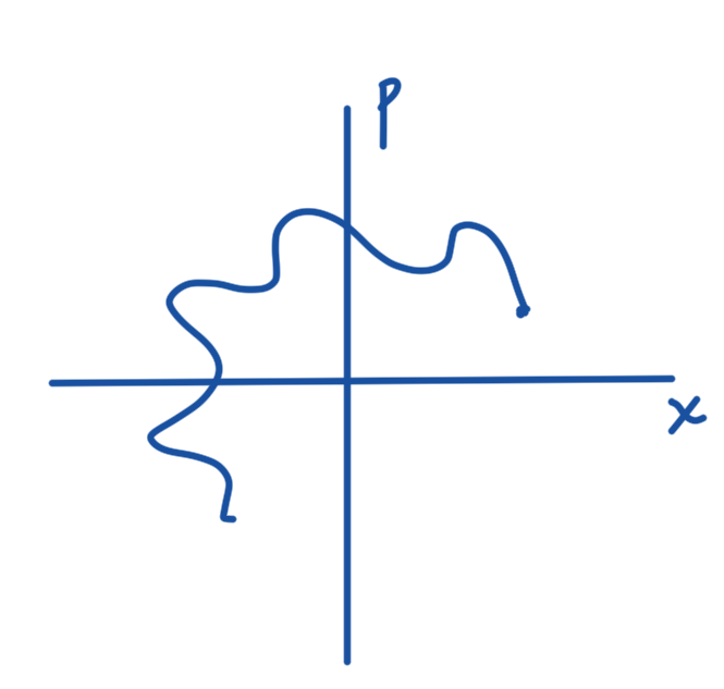
A two dimensional phase space as sketched in fig. 1 shows the trajectory of a point particle subject to some equations of motion

lectureOnePhaseSpaceClassicalFig1

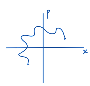
fig. 1. One dimensional classical phase space example

Quantum mechanics

For this lecture, we’ll work with natural units, setting

\begin{equation}\label{eqn:qmLecture1:480}
\boxed{
\Hbar = 1.
}
\end{equation}

In QM we are no longer allowed to think of position and momentum, but have to start asking about state vectors \( \ket{\Psi} \).

We’ll consider the state vector with respect to some basis, for example, in a position basis, we write

\begin{equation}\label{eqn:qmLecture1:40}
\braket{ x }{\Psi } = \Psi(x),
\end{equation}

a complex numbered “wave function”, the probability amplitude for a particle in \( \ket{\Psi} \) to be in the vicinity of \( x \).

We could also consider the state in a momentum basis

\begin{equation}\label{eqn:qmLecture1:60}
\braket{ p }{\Psi } = \Psi(p),
\end{equation}

a probability amplitude with respect to momentum \( p \).

More precisely,

\begin{equation}\label{eqn:qmLecture1:80}
\Abs{\Psi(x)}^2 dx \ge 0
\end{equation}

is the probability of finding the particle in the range \( (x, x + dx ) \). To have meaning as a probability, we require

\begin{equation}\label{eqn:qmLecture1:100}
\int_{-\infty}^\infty \Abs{\Psi(x)}^2 dx = 1.
\end{equation}

The average position can be calculated using this probability density function. For example

\begin{equation}\label{eqn:qmLecture1:120}
\expectation{x} = \int_{-\infty}^\infty \Abs{\Psi(x)}^2 x dx,
\end{equation}

or
\begin{equation}\label{eqn:qmLecture1:140}
\expectation{f(x)} = \int_{-\infty}^\infty \Abs{\Psi(x)}^2 f(x) dx.
\end{equation}

Similarly, calculation of an average of a function of momentum can be expressed as

\begin{equation}\label{eqn:qmLecture1:160}
\expectation{f(p)} = \int_{-\infty}^\infty \Abs{\Psi(p)}^2 f(p) dp.
\end{equation}

Transformation from a position to momentum basis

We have a problem, if we which to compute an average in momentum space such as \( \expectation{p} \), when given a wavefunction \( \Psi(x) \).

How do we convert

\begin{equation}\label{eqn:qmLecture1:180}
\Psi(p)
\stackrel{?}{\leftrightarrow}
\Psi(x),
\end{equation}

or equivalently
\begin{equation}\label{eqn:qmLecture1:200}
\braket{p}{\Psi}
\stackrel{?}{\leftrightarrow}
\braket{x}{\Psi}.
\end{equation}

Such a conversion can be performed by virtue of an the assumption that we have a complete orthonormal basis, for which we can introduce identity operations such as

\begin{equation}\label{eqn:qmLecture1:220}
\int_{-\infty}^\infty dp \ket{p}\bra{p} = 1,
\end{equation}

or
\begin{equation}\label{eqn:qmLecture1:240}
\int_{-\infty}^\infty dx \ket{x}\bra{x} = 1
\end{equation}

Some interpretations:

  1. \( \ket{x_0} \leftrightarrow \text{sits at} x = x_0 \)
  2. \( \braket{x}{x’} \leftrightarrow \delta(x – x’) \)
  3. \( \braket{p}{p’} \leftrightarrow \delta(p – p’) \)
  4. \( \braket{x}{p’} = \frac{e^{i p x}}{\sqrt{V}} \), where \( V \) is the volume of the box containing the particle. We’ll define the appropriate normalization for an infinite box volume later.

The delta function interpretation of the braket \( \braket{p}{p’} \) justifies the identity operator, since we recover any state in the basis when operating with it. For example, in momentum space

\begin{equation}\label{eqn:qmLecture1:260}
\begin{aligned}
1 \ket{p}
&=
\lr{ \int_{-\infty}^\infty dp’
\ket{p’}\bra{p’} }
\ket{p} \\
&=
\int_{-\infty}^\infty dp’
\ket{p’}
\braket{p’}{p} \\
&=
\int_{-\infty}^\infty dp’
\ket{p’}
\delta(p – p’) \\
&=
\ket{p}.
\end{aligned}
\end{equation}

This also the determination of an integral operator representation for the delta function

\begin{equation}\label{eqn:qmLecture1:500}
\begin{aligned}
\delta(x – x’)
&=
\braket{x}{x’} \\
&=
\int dp \braket{x}{p} \braket{p}{x’} \\
&=
\inv{V} \int dp e^{i p x} e^{-i p x’},
\end{aligned}
\end{equation}

or

\begin{equation}\label{eqn:qmLecture1:520}
\delta(x – x’)
=
\inv{V} \int dp e^{i p (x- x’)}.
\end{equation}

Here we used the fact that \( \braket{p}{x} = \braket{x}{p}^\conj \).

FIXME: do we have a justification for that conjugation with what was defined here so far?

The conversion from a position basis to momentum space is now possible

\begin{equation}\label{eqn:qmLecture1:280}
\begin{aligned}
\braket{p}{\Psi}
&= \Psi(p) \\
&= \int_{-\infty}^\infty \braket{p}{x} \braket{x}{\Psi} dx \\
&= \int_{-\infty}^\infty \frac{e^{-ip x}}{\sqrt{V}} \Psi(x) dx.
\end{aligned}
\end{equation}

The momentum space to position space conversion can be written as

\begin{equation}\label{eqn:qmLecture1:300}
\Psi(x)
= \int_{-\infty}^\infty \frac{e^{ip x}}{\sqrt{V}} \Psi(p) dp.
\end{equation}

Now we can go back and figure out the an expectation

\begin{equation}\label{eqn:qmLecture1:320}
\begin{aligned}
\expectation{p}
&=
\int \Psi^\conj(p) \Psi(p) p d p \\
&=
\int dp
\lr{
\int_{-\infty}^\infty \frac{e^{ip x}}{\sqrt{V}} \Psi^\conj(x) dx
}
\lr{
\int_{-\infty}^\infty \frac{e^{-ip x’}}{\sqrt{V}} \Psi(x’) dx’
}
p \\
&=\int dp dx dx’
\Psi^\conj(x)
\inv{V} e^{ip (x-x’)} \Psi(x’) p \\
&=
\int dp dx dx’
\Psi^\conj(x)
\inv{V} \lr{ -i\PD{x}{e^{ip (x-x’)}} }\Psi(x’) \\
&=
\int dp dx
\Psi^\conj(x) \lr{ -i \PD{x}{} }
\inv{V} \int dx’ e^{ip (x-x’)} \Psi(x’) \\
&=
\int dx
\Psi^\conj(x) \lr{ -i \PD{x}{} }
\int dx’ \lr{ \inv{V} \int dp e^{ip (x-x’)} } \Psi(x’) \\
&=
\int dx
\Psi^\conj(x) \lr{ -i \PD{x}{} }
\int dx’ \delta(x – x’) \Psi(x’) \\
&=
\int dx
\Psi^\conj(x) \lr{ -i \PD{x}{} }
\Psi(x)
\end{aligned}
\end{equation}

Here we’ve essentially calculated the position space representation of the momentum operator, allowing identifications of the following form

\begin{equation}\label{eqn:qmLecture1:380}
p \leftrightarrow -i \PD{x}{}
\end{equation}
\begin{equation}\label{eqn:qmLecture1:400}
p^2 \leftrightarrow – \PDSq{x}{}.
\end{equation}

Alternate starting point.

Most of the above results followed from the claim that \( \braket{x}{p} = e^{i p x} \). Note that this position space representation of the momentum operator can also be taken as the starting point. Given that, the exponential representation of the position-momentum braket follows

\begin{equation}\label{eqn:qmLecture1:540}
\bra{x} P \ket{p}
=
-i \Hbar \PD{x}{} \braket{x}{p},
\end{equation}

but \( \bra{x} P \ket{p} = p \braket{x}{p} \), providing a differential equation for \( \braket{x}{p} \)

\begin{equation}\label{eqn:qmLecture1:560}
p \braket{x}{p} = -i \Hbar \PD{x}{} \braket{x}{p},
\end{equation}

with solution

\begin{equation}\label{eqn:qmLecture1:580}
i p x/\Hbar = \ln \braket{x}{p} + \text{const},
\end{equation}

or
\begin{equation}\label{eqn:qmLecture1:600}
\braket{x}{p} \propto e^{i p x/\Hbar}.
\end{equation}

Matrix interpretation

  1. Ket’s \( \ket{\Psi} \leftrightarrow \text{column vector} \)
  2. Bra’s \( \bra{\Psi} \leftrightarrow {(\text{row vector})}^\conj \)
  3. Operators \( \leftrightarrow \) matrices that act on vectors.

\begin{equation}\label{eqn:qmLecture1:420}
\hat{p} \ket{\Psi} \rightarrow \ket{\Psi’}
\end{equation}

Time evolution

For a state subject to the equations of motion given by the Hamiltonian operator \( \hat{H} \)

\begin{equation}\label{eqn:qmLecture1:440}
i \PD{t}{} \ket{\Psi} = \hat{H} \ket{\Psi},
\end{equation}

the time evolution is given by
\begin{equation}\label{eqn:qmLecture1:460}
\ket{\Psi(t)} = e^{-i \hat{H} t} \ket{\Psi(0)}.
\end{equation}

Incomplete information

We’ll need to introduce the concept of Density matrices. This will bring us to concepts like entanglement.

References

[1] Jun John Sakurai and Jim J Napolitano. Modern quantum mechanics. Pearson Higher Ed, 2014.

Notes from reading Sakurai’s QM, prep for graduate Quantum Mechanics (PHY1520H)

September 14, 2015 phy1520 , ,

I start the lectures for grad Quantum Mechanics (PHY1520H) tomorrow, taught by Prof. Arun Paramekanti.

The curriculum has scary range of material, although some of it will be review. As prep for that, I’ve been working some problems, and have also explored a few interesting details and digressions. My notes for that preparatory work, collecting a number of individual posts from over the summer, is now posted.

Generalized Gaussian integrals

September 10, 2015 phy1520 , , , ,

[Click here for a PDF of this post with nicer formatting]

Both [3] and [4] use Gaussian integrals with both (negative) real, and imaginary arguments, which give the impression that the following is true:

\begin{equation}\label{eqn:generalizedGaussian:20}
\int_{-\infty}^\infty \exp\lr{ a x^2 } dx = \sqrt{\frac{-\pi}{a}},
\end{equation}

even when \( a \) is not a real negative constant, and in particular, with values \( a = \pm i \). Clearly this doesn’t follow by just making a substition \( x \rightarrow x/\sqrt{a} \), since that moves the integration range onto a rotated path in the complex plane when \( a \) is \( \pm i \). However, with some care, it can be shown that \ref{eqn:generalizedGaussian:20} holds provided \( \textrm{Re} \, a \le 0 \).

The first special case is \( \int_{-\infty}^\infty \exp\lr{ – x^2 } dx = \sqrt{\pi} \) which is easy to derive using the usual square it and integrate in circular coordinates trick.

Purely imaginary cases.

Let’s handle the \( a = \pm i \) cases next. These can be evaluated by considering integrals over the contours of fig. 1, where the upper plane contour is used for \( a = i \) and the lower plane contour for \( a = -i \).

twoContours45DegreesFig1

fig. 1. Contours for a = i,-i

Since there are no poles, the integral over either such contour is zero. Credit for figuring out how to tackle that integral and what contour to use goes to Dr MV, on stackexchange [2].

For the upper plane contour we have

\begin{equation}\label{eqn:generalizedGaussian:40}
\begin{aligned}
0
&= \oint \exp\lr{ i z^2 } dz \\
&= \int_0^R \exp\lr{ i x^2 } dx
+ \int_0^{\pi/4} \exp\lr{ i R^2 e^{2 i \theta} } R i e^{i\theta} d\theta
+ \int_R^0 \exp\lr{ i^2 t^2 } e^{i\pi/4} dt.
\end{aligned}
\end{equation}

Observe that \( i e^{2 i \theta} = i\cos(2 \theta) – \sin(2\theta) \) which has a negative real part for all values of \( \theta \ne 0 \). Provided the contour is slightly deformed from the axis, that second integral has a term of the form \( \sim R e^{-R^2} \) which tends to zero as \( R \rightarrow \infty \). So in the limit, this is

\begin{equation}\label{eqn:generalizedGaussian:60}
\int_0^\infty \exp\lr{ i x^2 } dx
= \sqrt{\pi} e^{i\pi/4}/2,
\end{equation}

or
\begin{equation}\label{eqn:generalizedGaussian:80}
\int_{-\infty}^\infty \exp\lr{ i x^2 } dx
= \sqrt{i \pi},
\end{equation}

a special case of \ref{eqn:generalizedGaussian:20} as desired. For \( a = -i \) integrating around the lower plane contour, we have

\begin{equation}\label{eqn:generalizedGaussian:100}
\begin{aligned}
0
&= \oint \exp\lr{ -i z^2 } dz \\
&= \int_0^R \exp\lr{ i x^2 } dx
+ \int_0^{-\pi/4} \exp\lr{ -i R^2 e^{2 i \theta} } R i e^{i\theta} d\theta
+ \int_R^0 \exp\lr{ -i (-i) t^2 } e^{-i\pi/4} dt.
\end{aligned}
\end{equation}

This time, in the second integral we also have \( -i R^2 e^{2 i \theta} = i R^2 \cos(2 \theta) + \sin(2 \theta) \), which also has a negative real part for \( \theta \in (0, \pi/4] \). Again the contour needs to be infinitesimally deformed, placed just lower than the axis.

This time we find

\begin{equation}\label{eqn:generalizedGaussian:120}
\int_{-\infty}^\infty \exp\lr{ -i x^2 } dx
= \sqrt{-i \pi},
\end{equation}

another special case of \ref{eqn:generalizedGaussian:20}.

Note.

Distorting the contour in this fashion seems somewhat like handwaving. A better approach would probably follow [1] where Jordan’s lemma is covered. It doesn’t look like Jordan’s lemma applies as is to this case, but the arguments look like they could be adapted appropriately.

Completely complex case.

A similar trick can be used to evaluate the more general cases, but a bit of thought is required to figure out the contours required. More precisely, while these contours will still have a wedge of pie shape, as sketched in fig. 2, we have to figure out the angle subtended by the edge of this piece of pie.

twoContoursThetaFig2

fig. 2. Contours for complex a.

To evaluate an integral consider

\begin{equation}\label{eqn:generalizedGaussian:140}
\begin{aligned}
0
&= \oint \exp\lr{ e^{i\phi} z^2 } dz \\
&= \int_0^R \exp\lr{ e^{i\phi} x^2 } dx
+ \int_0^{\theta} \exp\lr{ e^{i\phi} R^2 e^{2 i \mu} } R i e^{i\mu} d\mu
+ \int_R^0 \exp\lr{ e^{i\phi} e^{2 i \theta} t^2 } e^{i\theta} dt,
\end{aligned}
\end{equation}

where \( \phi \in (\pi/2, \pi) \cup (\pi,3\pi/2) \). We have a hope of evaluating this last integral if \( \phi + 2 \theta = \pi \), or

\begin{equation}\label{eqn:generalizedGaussian:160}
\theta = (\pi -\phi)/2,
\end{equation}

giving

\begin{equation}\label{eqn:generalizedGaussian:180}
\int_0^R \exp\lr{ e^{i\phi} x^2 } dx
=
e^{i\lr{\pi – \phi}/2} \int_0^R \exp\lr{ -t^2 } dt
– \int_0^{\theta} \exp\lr{ R^2 \lr{ \cos\lr{\phi + 2 \mu} + i \sin\lr{\phi + 2 \mu}} } R i e^{i\mu} d\mu.
\end{equation}

If the cosine is always negative on the chosen contours, then that integral will vanish in the \( R \rightarrow \infty \) limit. This turns out to be the case, which can be confirmed by considering each of the contours in sequence. If the upper plane contour is used to evaluate the integral for the \( \phi \in (\pi/2,\pi) \) case, we have

\begin{equation}\label{eqn:generalizedGaussian:200}
\theta \in (0, \pi/4).
\end{equation}

Since \( \phi + 2\theta = \pi \), we have

\begin{equation}\label{eqn:generalizedGaussian:220}
\phi + 2 \mu \in (\pi/2, \pi),
\end{equation}

and find that the cosine is strictly negative on that contour for that range of \( \phi \). Picking the lower plane contour for the \( \phi \in (\pi, 3\pi/2) \) range, we have

\begin{equation}\label{eqn:generalizedGaussian:240}
\theta \in (-\pi/4, 0),
\end{equation}

and so

\begin{equation}\label{eqn:generalizedGaussian:260}
\phi + 2 \mu \in (\pi/2, 3\pi/2).
\end{equation}

For this range of \( \phi \) the cosine on the lower plane contour is again negative as desired, so in the infinite \( R \) limit we have

\begin{equation}\label{eqn:generalizedGaussian:280}
\int_0^\infty \exp\lr{ e^{i\phi} x^2 } dx
=
\inv{2} \sqrt{ -\pi e^{-i\phi} }.
\end{equation}

The points at \( \phi = \pi/2, \pi, 3\pi/2 \) were omitted, but we’ve found the same result at those points, completing the verification of \ref{eqn:generalizedGaussian:20} for all \( \textrm{Re} a \le 0 \).

References

[1] W.R. Le Page and W.R. LePage. Complex Variables and the Laplace Transform for Engineers, chapter 8-10. A Theorem for Trigonometric Integrals. Courier Dover Publications, 1980.

[2] Dr. MV. Evaluating definite integral of exp(i t^2), 2015. URL https://math.stackexchange.com/a/1411084/359. [Online; accessed 10-September-2015].

[3] Jun John Sakurai and Jim J Napolitano. Modern quantum mechanics. Pearson Higher Ed, 2014.

[4] A. Zee. Quantum field theory in a nutshell. Universities Press, 2005.

Free particle propagator

September 7, 2015 phy1520 , , , , , ,

[Click here for a PDF of this post with nicer formatting]

Question: Free particle propagator ([1] pr. 2.31)

Derive the free particle propagator in one and three dimensions.

Answer

I found the description in the text confusing, so let’s start from scratch with the definition of the propagator. This is the kernel of the spatial convolution integral that encodes time evolution, and can be expressed by expanding a general time state with two sets of identity operators. Let the position relative state at time \( t \), relative to an initial time \( t_0 \) be given by \( \braket{\Bx}{\alpha, t ; t_0 } \), and expand this in terms of a complete basis of energy eigenstates \( | a’ > \) and the time evolution operator

\begin{equation}\label{eqn:freeParticlePropagator:20}
\begin{aligned}
\braket{\Bx”}{\alpha, t ; t_0 }
&= \bra{\Bx”} U \ket{\alpha, t_0 } \\
&= \bra{\Bx”} e^{-i H (t -t_0)/\Hbar} \ket{\alpha, t_0 } \\
&= \bra{\Bx”} e^{-i H (t -t_0)/\Hbar} \lr{ \sum_{a’} \ket{a’} \bra{a’ }} \ket{\alpha, t_0 } \\
&= \bra{\Bx”} \sum_{a’} e^{-i E_{a’} (t -t_0)/\Hbar} \ket{a’} \braket{a’ }{\alpha, t_0 } \\
&=
\bra{\Bx”} \sum_{a’} e^{-i E_{a’} (t -t_0)/\Hbar} \ket{a’} \bra{a’ }
\lr{ \int d^3 \Bx’
\ket{\Bx’}\bra{\Bx’}
}
\ket{\alpha, t_0 } \\
&=
\int d^3 \Bx’
\lr{
\bra{\Bx”} \sum_{a’} e^{-i E_{a’} (t -t_0)/\Hbar} \ket{a’} \braket{a’ }{\Bx’}
}
\braket{\Bx’}{\alpha, t_0 } \\
&=
\int d^3 \Bx’ K(\Bx”, t ; \Bx’, t_0) \braket{\Bx’}{\alpha, t_0 },
\end{aligned}
\end{equation}

where

\begin{equation}\label{eqn:freeParticlePropagator:40}
K(\Bx”, t ; \Bx’, t_0) =
\sum_{a’}
\braket{\Bx”}{a’}\braket{a’ }{\Bx’}
e^{-i E_{a’} (t -t_0)/\Hbar},
\end{equation}

the propagator, is the kernel of the convolution integral that takes the state \( \ket{\alpha, t_0} \) to state \( \ket{\alpha, t ; t_0} \). Evaluating this over the momentum states (where integration and not plain summation is required), we have

\begin{equation}\label{eqn:freeParticlePropagator:60}
\begin{aligned}
K(\Bx”, t ; \Bx’, t_0)
&=
\int d^3 \Bp’
\braket{\Bx”}{\Bp’}\braket{\Bp’ }{\Bx’}
e^{-i E_{\Bp’} (t -t_0)/\Hbar} \\
&=
\int d^3 \Bp’
\braket{\Bx”}{\Bp’}\braket{\Bp’ }{\Bx’}
\exp\lr{-i \frac{(\Bp’)^2 (t -t_0)}{2 m \Hbar}} \\
&=
\int d^3 \Bp’
\frac{e^{i \Bx” \cdot \Bp’/\Hbar}}{(\sqrt{2 \pi \Hbar})^3}
\frac{e^{-i \Bx’ \cdot \Bp’/\Hbar}}{(\sqrt{2 \pi \Hbar})^3}
\exp\lr{-i \frac{(\Bp’)^2 (t -t_0)}{2 m \Hbar}} \\
&=
\inv{(2 \pi \Hbar)^3}
\int d^3 \Bp’
e^{i (\Bx” -\Bx’) \cdot \Bp’/\Hbar}
\exp\lr{-i \frac{(\Bp’)^2 (t -t_0)}{2 m \Hbar}} \\
&=
\inv{ 2 \pi \Hbar }
\int_{-\infty}^\infty dp_1′
e^{i (x_1” -x_1′) p_1’/\Hbar}
\exp\lr{-i \frac{(p_1′)^2 (t -t_0)}{2 m \Hbar}} \times \\
&\quad \inv{ 2 \pi \Hbar }
\int_{-\infty}^\infty dp_2′
e^{i (x_2” -x_2′) p_2’/\Hbar}
\exp\lr{-i \frac{(p_2′)^2 (t -t_0)}{2 m \Hbar}} \times \\
&\quad \inv{ 2 \pi \Hbar }
\int_{-\infty}^\infty dp_3′
e^{i (x_3” -x_3′) p_3’/\Hbar}
\exp\lr{-i \frac{(p_3′)^2 (t -t_0)}{2 m \Hbar}}
\end{aligned}
\end{equation}

With \( a = \ifrac{(t -t_0)}{2 m \Hbar} \), each of these three integral factors is of the form

\begin{equation}\label{eqn:freeParticlePropagator:80}
\begin{aligned}
\inv{ 2 \pi \Hbar }
\int_{-\infty}^\infty dp
e^{i \Delta x p/\Hbar }
\exp\lr{-i a p^2}
&=
\inv{2 \pi \Hbar \sqrt{a}}
\int_{-\infty}^\infty du
e^{i \Delta x u/(\sqrt{a}\Hbar) }
\exp\lr{-i u^2} \\
&=
\inv{2 \pi \Hbar \sqrt{a}}
\int_{-\infty}^\infty du
e^{i \Delta x u/(\sqrt{a} \Hbar) }
\exp\lr{-i (u – \Delta x /(2\sqrt{a}\Hbar))^2 + i(\Delta x/(2\sqrt{a}\Hbar))^2} \\
&=
\inv{2 \pi \Hbar \sqrt{a}}
\exp\lr{ \frac{i(\Delta x)^2 2 m \Hbar}{4 (t -t_0) \Hbar^2} }
\int_{-\infty}^\infty dz
e^{-i z^2} \\
&= \sqrt{ \frac{ -i \pi 2 m \Hbar}{ 4 \pi^2 \Hbar^2 (t -t_0)} }
\exp\lr{ \frac{i(\Delta x)^2 m}{2 (t -t_0) \Hbar} } \\
&= \sqrt{ \frac{ m }{ 2 \pi i \Hbar (t -t_0)} }
\exp\lr{ \frac{i(\Delta x)^2 m}{2 (t -t_0) \Hbar} }.
\end{aligned}
\end{equation}

Note that the integral above has value \( \sqrt{-i\pi} \) which can be found by integrating over the contour of fig. 1, letting \( R \rightarrow \infty \).

contourFig1

fig. 1. Integration contour for \( \int e^{-i z^2} \)

Multiplying out each of the spatial direction factors gives the propagator in its closed form
\begin{equation}\label{eqn:freeParticlePropagator:120}
\boxed{
K(\Bx”, t ; \Bx’, t_0)
= \lr{ \sqrt{ \frac{ m }{ 2 \pi i \Hbar (t -t_0)} } }^3
\exp\lr{ \frac{i(\Bx” – \Bx’)^2 m}{2 (t -t_0) \Hbar} }.
}
\end{equation}

In one or two dimensions the exponential power \( 3 \) need only be adjusted appropriately.

Question: Momentum space free particle propagator ([1] pr. 2.33)

Derive the free particle propagator in momentum space.

Answer

The momentum space propagator follows in the same fashion as the spatial propagator

\begin{equation}\label{eqn:freeParticlePropagator:140}
\begin{aligned}
\braket{\Bp”}{\alpha, t ; t_0 }
&= \bra{\Bp”} U \ket{\alpha, t_0 } \\
&= \bra{\Bp”} e^{-i H (t -t_0)/\Hbar} \ket{\alpha, t_0 } \\
&= \bra{\Bp”} e^{-i H (t -t_0)/\Hbar} \lr{ \sum_{a’} \ket{a’} \bra{a’ }} \ket{\alpha, t_0 } \\
&= \bra{\Bp”} \sum_{a’} e^{-i E_{a’} (t -t_0)/\Hbar} \ket{a’} \braket{a’ }{\alpha, t_0 } \\
&=
\bra{\Bp”} \sum_{a’} e^{-i E_{a’} (t -t_0)/\Hbar} \ket{a’} \bra{a’ }
\lr{ \int d^3 \Bp’
\ket{\Bp’}\bra{\Bp’}
}
\ket{\alpha, t_0 } \\
&=
\int d^3 \Bp’
\lr{
\bra{\Bp”} \sum_{a’} e^{-i E_{a’} (t -t_0)/\Hbar} \ket{a’} \braket{a’ }{\Bp’}
}
\braket{\Bp’}{\alpha, t_0 } \\
&=
\int d^3 \Bp’ K(\Bp”, t ; \Bp’, t_0) \braket{\Bp’}{\alpha, t_0 },
\end{aligned}
\end{equation}

so

\begin{equation}\label{eqn:freeParticlePropagator:160}
K(\Bp”, t ; \Bp’, t_0)
=
\sum_{a’}
\braket{\Bp”}{a’}
\braket{a’ }{\Bp’}
e^{-i E_{a’} (t -t_0)/\Hbar}.
\end{equation}

For the free particle Hamiltonian, this can be evaluated over a momentum space basis

\begin{equation}\label{eqn:freeParticlePropagator:170}
\begin{aligned}
K(\Bp”, t ; \Bp’, t_0)
&=
\int d^3 \Bp”’
\braket{\Bp”}{\Bp”’}
\braket{\Bp”’ }{\Bp’}
e^{-i E_{\Bp”’} (t -t_0)/\Hbar} \\
&=
\int d^3 \Bp”’
\braket{\Bp”}{\Bp”’}
\delta(\Bp”’ – \Bp’)
\exp\lr{ -i \frac{(\Bp”’)^2 (t -t_0)}{2 m \Hbar}} \\
&=
\braket{\Bp”}{\Bp’}
\exp\lr{ -i \frac{(\Bp’)^2 (t -t_0)}{2 m \Hbar}}
\end{aligned}
\end{equation}

or

\begin{equation}\label{eqn:freeParticlePropagator:200}
\boxed{
K(\Bp”, t ; \Bp’, t_0)
=
\delta( \Bp” – \Bp’ )
\exp\lr{ -i \frac{(\Bp’)^2 (t -t_0)}{2 m \Hbar}}.
}
\end{equation}

This is what we expect since the time evolution is given by just this exponential factor

\begin{equation}\label{eqn:freeParticlePropagator:220}
\begin{aligned}
\braket{\Bp’}{\alpha, t_0 ; t}
&= \bra{\Bp’} \exp\lr{ -i \frac{(\Bp’)^2 (t -t_0)}{2 m \Hbar}} \ket{\alpha, t_0} \\
&=
\exp\lr{ -i \frac{(\Bp’)^2 (t -t_0)}{2 m \Hbar}}
\braket{\Bp’}
{\alpha, t_0}.
\end{aligned}
\end{equation}

References

[1] Jun John Sakurai and Jim J Napolitano. Modern quantum mechanics. Pearson Higher Ed, 2014.