phy2403

PHY2403H Quantum Field Theory. Lecture 3: Lorentz transformations and a scalar action. Taught by Prof. Erich Poppitz

September 18, 2018 phy2403 , ,

[Click here for a PDF of this post with nicer formatting]

DISCLAIMER: Very rough notes from class. Some additional side notes, but otherwise barely edited.

These are notes for the UofT course PHY2403H, Quantum Field Theory, taught by Prof. Erich Poppitz.

Determinant of Lorentz transformations

We require that Lorentz transformations leave the dot product invariant, that is \( x \cdot y = x’ \cdot y’ \), or
\begin{equation}\label{eqn:qftLecture3:20}
x^\mu g_{\mu\nu} y^\nu = {x’}^\mu g_{\mu\nu} {y’}^\nu.
\end{equation}
Explicitly, with coordinate transformations
\begin{equation}\label{eqn:qftLecture3:40}
\begin{aligned}
{x’}^\mu &= {\Lambda^\mu}_\rho x^\rho \\
{y’}^\mu &= {\Lambda^\mu}_\rho y^\rho
\end{aligned}
\end{equation}
such a requirement is equivalent to demanding that
\begin{equation}\label{eqn:qftLecture3:500}
\begin{aligned}
x^\mu g_{\mu\nu} y^\nu
&=
{\Lambda^\mu}_\rho x^\rho
g_{\mu\nu}
{\Lambda^\nu}_\kappa y^\kappa \\
&=
x^\mu
{\Lambda^\alpha}_\mu
g_{\alpha\beta}
{\Lambda^\beta}_\nu
y^\nu,
\end{aligned}
\end{equation}
or
\begin{equation}\label{eqn:qftLecture3:60}
g_{\mu\nu}
=
{\Lambda^\alpha}_\mu
g_{\alpha\beta}
{\Lambda^\beta}_\nu
\end{equation}

multiplying by the inverse we find
\begin{equation}\label{eqn:qftLecture3:200}
\begin{aligned}
g_{\mu\nu}
{\lr{\Lambda^{-1}}^\nu}_\lambda
&=
{\Lambda^\alpha}_\mu
g_{\alpha\beta}
{\Lambda^\beta}_\nu
{\lr{\Lambda^{-1}}^\nu}_\lambda \\
&=
{\Lambda^\alpha}_\mu
g_{\alpha\lambda} \\
&=
g_{\lambda\alpha}
{\Lambda^\alpha}_\mu.
\end{aligned}
\end{equation}
This is now amenable to expressing in matrix form
\begin{equation}\label{eqn:qftLecture3:220}
\begin{aligned}
(G \Lambda^{-1})_{\mu\lambda}
&=
(G \Lambda)_{\lambda\mu} \\
&=
((G \Lambda)^\T)_{\mu\lambda} \\
&=
(\Lambda^\T G)_{\mu\lambda},
\end{aligned}
\end{equation}
or
\begin{equation}\label{eqn:qftLecture3:80}
G \Lambda^{-1}
=
(G \Lambda)^\T.
\end{equation}

Taking determinants (using the normal identities for products of determinants, determinants of transposes and inverses), we find
\begin{equation}\label{eqn:qftLecture3:100}
det(G)
det(\Lambda^{-1})
=
det(G) det(\Lambda),
\end{equation}
or
\begin{equation}\label{eqn:qftLecture3:120}
det(\Lambda)^2 = 1,
\end{equation}
or
\( det(\Lambda)^2 = \pm 1 \). We will generally ignore the case of reflections in spacetime that have a negative determinant.

Smart-alec Peeter pointed out after class last time that we can do the same thing easier in matrix notation
\begin{equation}\label{eqn:qftLecture3:140}
\begin{aligned}
x’ &= \Lambda x \\
y’ &= \Lambda y
\end{aligned}
\end{equation}
where
\begin{equation}\label{eqn:qftLecture3:160}
\begin{aligned}
x’ \cdot y’
&=
(x’)^\T G y’ \\
&=
x^\T \Lambda^\T G \Lambda y,
\end{aligned}
\end{equation}
which we require to be \( x \cdot y = x^\T G y \) for all four vectors \( x, y \), that is
\begin{equation}\label{eqn:qftLecture3:180}
\Lambda^\T G \Lambda = G.
\end{equation}
We can find the result \ref{eqn:qftLecture3:120} immediately without having to first translate from index notation to matrices.

Field theory

The electrostatic potential is an example of a scalar field \( \phi(\Bx) \) unchanged by SO(3) rotations
\begin{equation}\label{eqn:qftLecture3:240}
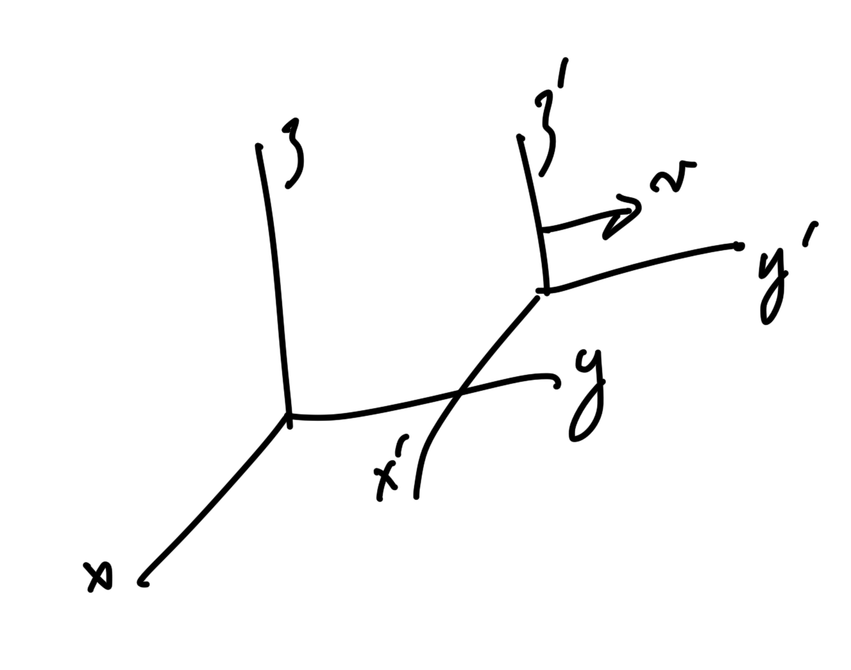
\Bx \rightarrow \Bx’ = O \Bx,
\end{equation}
that is
\begin{equation}\label{eqn:qftLecture3:260}
\phi'(\Bx’) = \phi(\Bx).
\end{equation}
Here \( \phi'(\Bx’) \) is the value of the (electrostatic) scalar potential in a primed frame.

However, the electrostatic field is not invariant under Lorentz transformation.
We postulate that there is some scalar field
\begin{equation}\label{eqn:qftLecture3:280}
\phi'(x’) = \phi(x),
\end{equation}
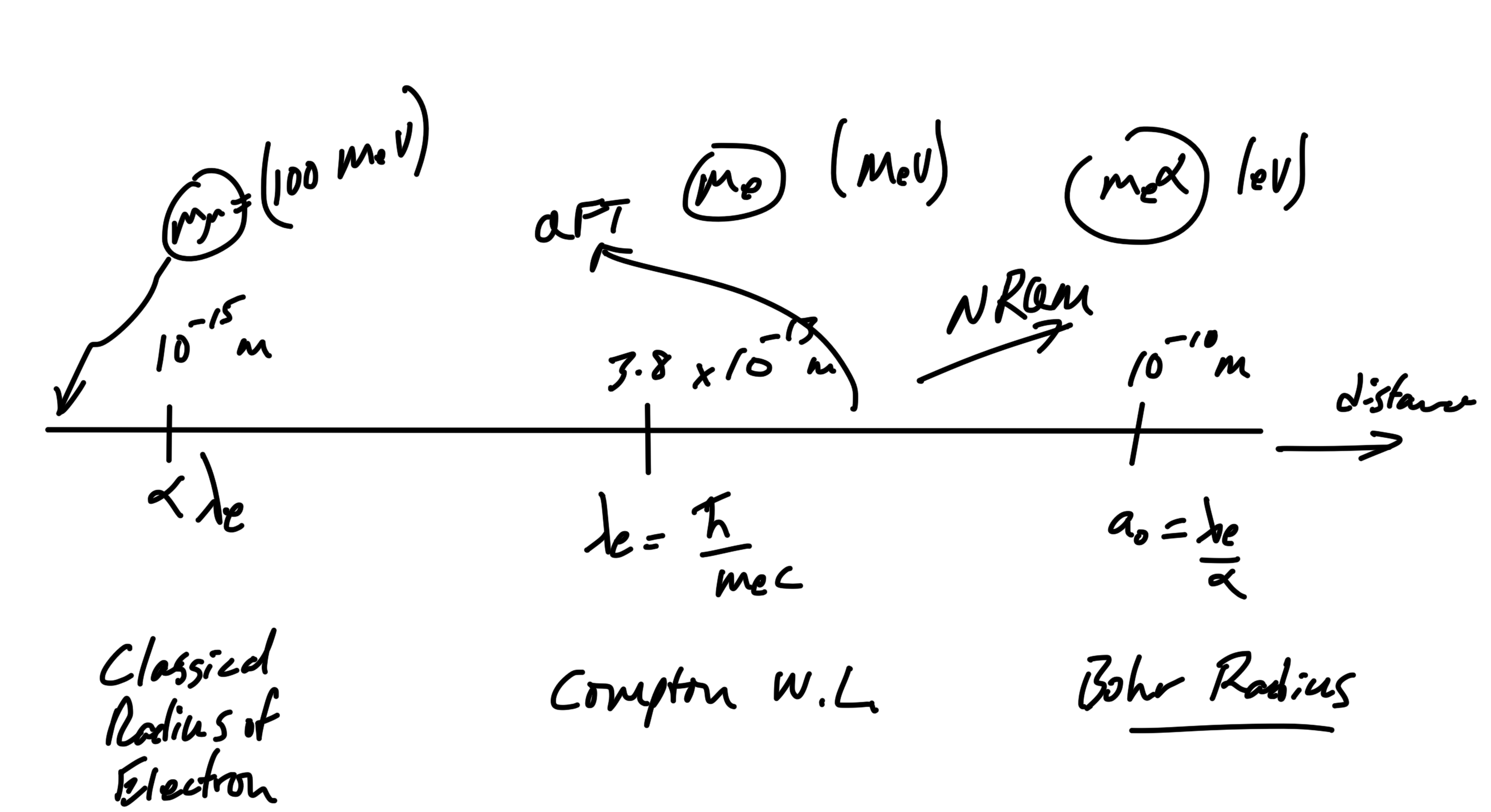
where \( x’ = \Lambda x \) is an SO(1,3) transformation. There are actually no stable particles (fields that persist at long distances) described by Lorentz scalar fields, although there are some unstable scalar fields such as the Higgs, Pions, and Kaons. However, much of our homework and discussion will be focused on scalar fields, since they are the easiest to start with.

We need to first understand how derivatives \( \partial_\mu \phi(x) \) transform. Using the chain rule
\begin{equation}\label{eqn:qftLecture3:300}
\begin{aligned}
\PD{x^\mu}{\phi(x)}
&=
\PD{x^\mu}{\phi'(x’)} \\
&=
\PD{{x’}^\nu}{\phi'(x’)}
\PD{{x}^\mu}{{x’}^\nu} \\
&=
\PD{{x’}^\nu}{\phi'(x’)}
\partial_\mu \lr{
{\Lambda^\nu}_\rho x^\rho
} \\
&=
\PD{{x’}^\nu}{\phi'(x’)}
{\Lambda^\nu}_\mu \\
&=
\PD{{x’}^\nu}{\phi(x)}
{\Lambda^\nu}_\mu.
\end{aligned}
\end{equation}
Multiplying by the inverse \( {\lr{\Lambda^{-1}}^\mu}_\kappa \) we get
\begin{equation}\label{eqn:qftLecture3:320}
\PD{{x’}^\kappa}{}
=
{\lr{\Lambda^{-1}}^\mu}_\kappa \PD{x^\mu}{}
\end{equation}

This should be familiar to you, and is an analogue of the transformation of the
\begin{equation}\label{eqn:qftLecture3:340}
d\Br \cdot \spacegrad_\Br
=
d\Br’ \cdot \spacegrad_{\Br’}.
\end{equation}

Actions

We will start with a classical action, and quantize to determine a QFT. In mechanics we have the particle position \( q(t) \), which is a classical field in 1+0 time and space dimensions. Our action is
\begin{equation}\label{eqn:qftLecture3:360}
S
= \int dt \LL(t)
= \int dt \lr{
\inv{2} \dot{q}^2 – V(q)
}.
\end{equation}
This action depends on the position of the particle that is local in time. You could imagine that we have a more complex action where the action depends on future or past times
\begin{equation}\label{eqn:qftLecture3:380}
S
= \int dt’ q(t’) K( t’ – t ),
\end{equation}
but we don’t seem to find such actions in classical mechanics.

Principles determining the form of the action.

  • relativity (action is invariant under Lorentz transformation)
  • locality (action depends on fields and the derivatives at given \((t, \Bx)\).
  • Gauge principle (the action should be invariant under gauge transformation). We won’t discuss this in detail right now since we will start with studying scalar fields.
    Recall that for Maxwell’s equations a gauge transformation has the form
    \begin{equation}\label{eqn:qftLecture3:520}
    \phi \rightarrow \phi + \dot{\chi}, \BA \rightarrow \BA – \spacegrad \chi.
    \end{equation}

Suppose we have a real scalar field \( \phi(x) \) where \( x \in \mathbb{R}^{1,d-1} \). We will be integrating over space and time \( \int dt d^{d-1} x \) which we will write as \( \int d^d x \). Our action is
\begin{equation}\label{eqn:qftLecture3:400}
S = \int d^d x \lr{ \text{Some action density to be determined } }
\end{equation}
The analogue of \( \dot{q}^2 \) is
\begin{equation}\label{eqn:qftLecture3:420}
\begin{aligned}
\lr{ \PD{x^\mu}{\phi} }
\lr{ \PD{x^\nu}{\phi} }
g^{\mu\nu}
&=
(\partial_\mu \phi) (\partial_\nu \phi) g^{\mu\nu} \\
&= \partial^\mu \phi \partial_\mu \phi.
\end{aligned}
\end{equation}
This has both time and spatial components, that is
\begin{equation}\label{eqn:qftLecture3:440}
\partial^\mu \phi \partial_\mu \phi =
\dotphi^2 – (\spacegrad \phi)^2,
\end{equation}
so the desired simplest scalar action is
\begin{equation}\label{eqn:qftLecture3:460}
S = \int d^d x \lr{ \dotphi^2 – (\spacegrad \phi)^2 }.
\end{equation}
The measure transforms using a Jacobian, which we have seen is the Lorentz transform matrix, and has unit determinant
\begin{equation}\label{eqn:qftLecture3:480}
d^d x’ = d^d x \Abs{ det( \Lambda^{-1} ) } = d^d x.
\end{equation}

Problems.

Question: Four vector form of the Maxwell gauge transformation.

Show that the transformation
\begin{equation}\label{eqn:qftLecture3:580}
A^\mu \rightarrow A^\mu + \partial^\mu \chi
\end{equation}
is the desired four-vector form of the gauge transformation \ref{eqn:qftLecture3:520}, that is
\begin{equation}\label{eqn:qftLecture3:540}
\begin{aligned}
j^\nu
&= \partial_\mu {F’}^{\mu\nu} \\
&= \partial_\mu F^{\mu\nu}.
\end{aligned}
\end{equation}
Also relate this four-vector gauge transformation to the spacetime split.

Answer

\begin{equation}\label{eqn:qftLecture3:560}
\begin{aligned}
\partial_\mu {F’}^{\mu\nu}
&=
\partial_\mu \lr{ \partial^\mu {A’}^\nu – \partial_\nu {A’}^\mu } \\
&=
\partial_\mu \lr{
\partial^\mu \lr{ A^\nu + \partial^\nu \chi }
– \partial_\nu \lr{ A^\mu + \partial^\mu \chi }
} \\
&=
\partial_\mu {F}^{\mu\nu}
+
\partial_\mu \partial^\mu \partial^\nu \chi

\partial_\mu \partial^\nu \partial^\mu \chi \\
&=
\partial_\mu {F}^{\mu\nu},
\end{aligned}
\end{equation}
by equality of mixed partials. Expanding \ref{eqn:qftLecture3:580} explicitly we find
\begin{equation}\label{eqn:qftLecture3:600}
{A’}^\mu = A^\mu + \partial^\mu \chi,
\end{equation}
which is
\begin{equation}\label{eqn:qftLecture3:620}
\begin{aligned}
\phi’ = {A’}^0 &= A^0 + \partial^0 \chi = \phi + \dot{\chi} \\
\BA’ \cdot \Be_k = {A’}^k &= A^k + \partial^k \chi = \lr{ \BA – \spacegrad \chi } \cdot \Be_k.
\end{aligned}
\end{equation}
The last of which can be written in vector notation as \( \BA’ = \BA – \spacegrad \chi \).

UofT QFT Fall 2018 Lecture 2. Units, scales, and Lorentz transformations. Taught by Prof. Erich Poppitz

September 17, 2018 phy2403 , , ,

[Click here for a PDF of this post with nicer formatting]

DISCLAIMER: Very rough notes from class. Some additional side notes, but otherwise barely edited.

Natural units.

\begin{equation}\label{eqn:qftLecture2:20}
\begin{aligned}
[\Hbar] &= [\text{action}] = M \frac{L^2}{T^2} T = \frac{M L^2}{T} \\
&= [\text{velocity}] = \frac{L}{T} \\
& [\text{energy}] = M \frac{L^2}{T^2}.
\end{aligned}
\end{equation}

Setting \( c = 1 \) means
\begin{equation}\label{eqn:qftLecture2:240}
\frac{L}{T} = 1
\end{equation}
and setting \( \Hbar = 1 \) means
\begin{equation}\label{eqn:qftLecture2:260}
[\Hbar] = [\text{action}] = M L {\frac{L}{T}} = M L
\end{equation}
therefore
\begin{equation}\label{eqn:qftLecture2:280}
[L] = \inv{\text{mass}}
\end{equation}
and
\begin{equation}\label{eqn:qftLecture2:300}
[\text{energy}] = M {\frac{L^2}{T^2}} = \text{mass}\, \text{eV}
\end{equation}

Summary

  • \( \text{energy} \sim \text{eV} \)
  • \( \text{distance} \sim \inv{M} \)
  • \( \text{time} \sim \inv{M} \)

From:
\begin{equation}\label{eqn:qftLecture2:320}
\alpha = \frac{e^2}{4 \pi {\Hbar c}}
\end{equation}
which is dimensionless (\(1/137\)), so electric charge is dimensionless.

Some useful numbers in natural units

\begin{equation}\label{eqn:qftLecture2:40}
\begin{aligned}
m_\txte &\sim 10^{-27} \text{g} \sim 0.5 \text{MeV} \\
m_\txtp &\sim 2000 m_\txte \sim 1 \text{GeV} \\
m_\pi &\sim 140 \text{MeV} \\
m_\mu &\sim 105 \text{MeV} \\
\Hbar c &\sim 200 \text{MeV} \,\text{fm} = 1
\end{aligned}
\end{equation}

Gravity

Interaction energy of two particles

\begin{equation}\label{eqn:qftLecture2:60}
G_\txtN \frac{m_1 m_2}{r}
\end{equation}

\begin{equation}\label{eqn:qftLecture2:80}
[\text{energy}] \sim [G_\txtN] \frac{M^2}{L}
\end{equation}

\begin{equation}\label{eqn:qftLecture2:100}
[G_\txtN]
\sim
[\text{energy}] \frac{L}{M^2}
\end{equation}

but energy x distance is dimensionless (action) in our units

\begin{equation}\label{eqn:qftLecture2:120}
[G_\txtN]
\sim
{\text{dimensionless}}{M^2}
\end{equation}

\begin{equation}\label{eqn:qftLecture2:140}
\frac{G_\txtN}{\Hbar c} \sim \inv{M^2} \sim \frac{1}{10^{20} \text{GeV}}
\end{equation}

Planck mass

\begin{equation}\label{eqn:qftLecture2:160}
M_{\text{Planck}} \sim \sqrt{\frac{\Hbar c}{G_\txtN}}
\sim 10^{-4} g \sim \inv{\lr{10^{20} \text{GeV}}^2}
\end{equation}

We can revisit the scale diagram from last lecture in terms of MeV mass/energy values, as sketched in fig. 1.

fig. 1. Scales, take II.

At the classical electron radius scale, we consider phenomena such as back reaction of radiation, the self energy of electrons. At the Compton wavelength we have to allow for production of multiple particle pairs. At Bohr radius scales we must start using QM instead of classical mechanics.

Cross section.

Verbal discussion of cross section, not captured in these notes. Roughly, the cross section sounds like the number of events per unit time, related to the flux of some source through an area.

We’ll compute the cross section of a number of different systems in this course. The cross section is relevant in scattering such as the electron-electron scattering sketched in fig. 2.

fig. 2. Electron electron scattering.

We assume that QED is highly relativistic. In natural units, our scale factor is basically the square of the electric charge
\begin{equation}\label{eqn:qftLecture2:180}
\alpha \sim e^2,
\end{equation}
so the cross section has the form
\begin{equation}\label{eqn:qftLecture2:200}
\sigma \sim \frac{\alpha^2}{E^2} \lr{ 1 + O(\alpha) + O(\alpha^2) + \cdots }
\end{equation}

In gravity we could consider scattering of electrons, where \( G_\txtN \) takes the place of \( \alpha \). However, \( G_\txtN \) has dimensions.

For electron-electron scattering due to gravitons

\begin{equation}\label{eqn:qftLecture2:220}
\sigma \sim \frac{G_\txtN^2 E^2}{1 + G_\txtN E^2 + \cdots }
\end{equation}

Now the cross section grows with energy. This will cause some problems (violating unitarity: probabilities greater than 1!) when \( O(G_\txtN E^2) = 1 \).

In any quantum field theories when the coupling constant is not-dimensionless we have the same sort of problems at some scale.

The point is that we can get far considering just dimensional analysis.

If the coupling constant has a dimension \((1/\text{mass})^N\,, N > 0\), then unitarity will be violated at high energy. One such theory is the Fermi theory of beta decay (electro-weak theory), which had a coupling constant with dimensions inverse-mass-squared. The relevant scale for beta decay was 4 Fermi, or \( G_\txtF \sim (1/{100 \text{GeV}})^2 \). This was the motivation for introducing the Higgs theory, which was motivated by restoring unitarity.

Lorentz transformations.

The goal, perhaps not for today, is to study the simplest (relativistic) scalar field theory. First studied classically, and then consider such a quantum field theory.

How is relativity implemented when we write the Lagrangian and action?

Our first step must be to consider Lorentz transformations and the Lorentz group.

Spacetime (Minkowski space) is \R{3,1} (or \R{d-1,1}). Our coordinates are

\begin{equation}\label{eqn:qftLecture2:340}
(c t, x^1, x^2, x^3) = (c t, \Br).
\end{equation}

Here, we’ve scaled the time scale by \( c \) so that we measure time and space in the same dimensions. We write this as

\begin{equation}\label{eqn:qftLecture2:360}
x^\mu = (x^0, x^1, x^2, x^3),
\end{equation}

where \( \mu = 0, 1, 2, 3 \), and call this a “4-vector”. These are called the space-time coordinates of an event, which tell us where and when an event occurs.

For two events whose spacetime coordinates differ by \( dx^0, dx^1, dx^2, dx^3 \) we introduce the notion of a space time \underline{interval}

\begin{equation}\label{eqn:qftLecture2:380}
\begin{aligned}
ds^2
&= c^2 dt^2
– (dx^1)^2
– (dx^2)^2
– (dx^3)^2 \\
&=
\sum_{\mu, \nu = 0}^3 g_{\mu\nu} dx^\mu dx^\nu
\end{aligned}
\end{equation}

Here \( g_{\mu\nu} \) is the Minkowski space metric, an object with two indexes that run from 0-3. i.e. this is a diagonal matrix

\begin{equation}\label{eqn:qftLecture2:400}
g_{\mu\nu} \sim
\begin{bmatrix}
1 & 0 & 0 & 0 \\
0 & -1 & 0 & 0 \\
0 & 0 & -1 & 0 \\
0 & 0 & 0 & -1 \\
\end{bmatrix}
\end{equation}

i.e.
\begin{equation}\label{eqn:qftLecture2:420}
\begin{aligned}
g_{00} &= 1 \\
g_{11} &= -1 \\
g_{22} &= -1 \\
g_{33} &= -1 \\
\end{aligned}
\end{equation}

We will use the Einstein summation convention, where any repeated upper and lower indexes are considered summed over. That is \ref{eqn:qftLecture2:380} is written with an implied sum
\begin{equation}\label{eqn:qftLecture2:440}
ds^2 = g_{\mu\nu} dx^\mu dx^\nu.
\end{equation}

Explicit expansion:
\begin{equation}\label{eqn:qftLecture2:460}
\begin{aligned}
ds^2
&= g_{\mu\nu} dx^\mu dx^\nu \\
&=
g_{00} dx^0 dx^0
+g_{11} dx^1 dx^1
+g_{22} dx^2 dx^2
+g_{33} dx^3 dx^3
&=
(1) dx^0 dx^0
+ (-1) dx^1 dx^1
+ (-1) dx^2 dx^2
+ (-1) dx^3 dx^3.
\end{aligned}
\end{equation}

Recall that rotations (with orthogonal matrix representations) are transformations that leave the dot product unchanged, that is

\begin{equation}\label{eqn:qftLecture2:480}
\begin{aligned}
(R \Bx) \cdot (R \By)
&= \Bx^\T R^\T R \By \\
&= \Bx^\T \By \\
&= \Bx \cdot \By,
\end{aligned}
\end{equation}

where \( R \) is a rotation orthogonal 3×3 matrix. The set of such transformations that leave the dot product unchanged have orthonormal matrix representations \( R^\T R = 1 \). We call the set of such transformations that have unit determinant the SO(3) group.

We call a Lorentz transformation, if it is a linear transformation acting on 4 vectors that leaves the spacetime interval (i.e. the inner product of 4 vectors) invariant. That is, a transformation that leaves
\begin{equation}\label{eqn:qftLecture2:500}
x^\mu y^\nu g_{\mu\nu} = x^0 y^0 – x^1 y^1 – x^2 y^2 – x^3 y^3
\end{equation}
unchanged.

Suppose that transformation has a 4×4 matrix form

\begin{equation}\label{eqn:qftLecture2:520}
{x’}^\mu = {\Lambda^\mu}_\nu x^\nu
\end{equation}

For an example of a possible \( \Lambda \), consider the transformation sketched in fig. 3.

fig. 3. Boost transformation.

We know that boost has the form
\begin{equation}\label{eqn:qftLecture2:540}
\begin{aligned}
x &= \frac{x’ + v t’}{\sqrt{1 – v^2/c^2}} \\
y &= y’ \\
z &= z’ \\
t &= \frac{t’ + (v/c^2) x’}{\sqrt{1 – v^2/c^2}} \\
\end{aligned}
\end{equation}
(this is a boost along the x-axis, not y as I’d drawn),
or
\begin{equation}\label{eqn:qftLecture2:560}
\begin{bmatrix}
c t \\
x \\
y \\
z
\end{bmatrix}
=
\begin{bmatrix}
\inv{\sqrt{1 – v^2/c^2}} & \frac{v/c}{\sqrt{1 – v^2/c^2}} & 0 & 0 \\
\frac{v/c}{\sqrt{1 – v^2/c^2}} & \frac{1}{\sqrt{1 – v^2/c^2}} & 0 & 0 \\
0 & 0 & 1 & 0 \\
0 & 0 & 0 & 1 \\
\end{bmatrix}
\begin{bmatrix}
c t’ \\
x’ \\
y’ \\
z’
\end{bmatrix}
\end{equation}

Other examples include rotations (\({\lambda^0}_0 = 1\) zeros in \( {\lambda^0}_k, {\lambda^k}_0 \), and a rotation matrix in the remainder.)

Back to Lorentz transformations (\(\text{SO}(1,3)^+\)), let
\begin{equation}\label{eqn:qftLecture2:600}
\begin{aligned}
{x’}^\mu &= {\Lambda^\mu}_\nu x^\nu \\
{y’}^\kappa &= {\Lambda^\kappa}_\rho y^\rho
\end{aligned}
\end{equation}

The dot product
\begin{equation}\label{eqn:qftLecture2:620}
g_{\mu \kappa}
{x’}^\mu
{y’}^\kappa
=
g_{\mu \kappa}
{\Lambda^\mu}_\nu
{\Lambda^\kappa}_\rho
x^\nu
y^\rho
=
g_{\nu\rho}
x^\nu
y^\rho,
\end{equation}
where the last step introduces the invariance requirement of the transformation. That is

\begin{equation}\label{eqn:qftLecture2:640}
\boxed{
g_{\nu\rho}
=
g_{\mu \kappa}
{\Lambda^\mu}_\nu
{\Lambda^\kappa}_\rho.
}
\end{equation}

Upper and lower indexes

We’ve defined

\begin{equation}\label{eqn:qftLecture2:660}
x^\mu = (t, x^1, x^2, x^3)
\end{equation}

We could also define a four vector with lower indexes
\begin{equation}\label{eqn:qftLecture2:680}
x_\nu = g_{\nu\mu} x^\mu = (t, -x^1, -x^2, -x^3).
\end{equation}
That is
\begin{equation}\label{eqn:qftLecture2:700}
\begin{aligned}
x_0 &= x^0 \\
x_1 &= -x^1 \\
x_2 &= -x^2 \\
x_3 &= -x^3.
\end{aligned}
\end{equation}

which allows us to write the dot product as simply \( x^\mu y_\mu \).

We can also define a metric tensor with upper indexes

\begin{equation}\label{eqn:qftLecture2:401}
g^{\mu\nu} \sim
\begin{bmatrix}
1 & 0 & 0 & 0 \\
0 & -1 & 0 & 0 \\
0 & 0 & -1 & 0 \\
0 & 0 & 0 & -1 \\
\end{bmatrix}
\end{equation}
This is the inverse matrix of \( g_{\mu\nu} \), and it satisfies
\begin{equation}\label{eqn:qftLecture2:720}
g^{\mu \nu} g_{\nu\rho} = {\delta^\mu}_\rho
\end{equation}

Exercise: Check:
\begin{equation}\label{eqn:qftLecture2:740}
\begin{aligned}
g_{\mu\nu} x^\mu y^\nu
&= x_\nu y^\nu \\
&= x^\nu y_\nu \\
&= g^{\mu\nu} x_\mu y_\nu \\
&= {\delta^\mu}_\nu x_\mu y^\nu.
\end{aligned}
\end{equation}

Class ended around this point, but it appeared that we were heading this direction:

Returning to the Lorentz invariant and multiplying both sides of
\ref{eqn:qftLecture2:640} with an inverse Lorentz transformation \( \Lambda^{-1} \), we find
\begin{equation}\label{eqn:qftLecture2:760}
\begin{aligned}
g_{\nu\rho}
{\lr{\Lambda^{-1}}^\rho}_\alpha
&=
g_{\mu \kappa}
{\Lambda^\mu}_\nu
{\Lambda^\kappa}_\rho
{\lr{\Lambda^{-1}}^\rho}_\alpha \\
&=
g_{\mu \kappa}
{\Lambda^\mu}_\nu
{\delta^\kappa}_\alpha \\
&=
g_{\mu \alpha}
{\Lambda^\mu}_\nu,
\end{aligned}
\end{equation}
or
\begin{equation}\label{eqn:qftLecture2:780}
\lr{\Lambda^{-1}}_{\nu \alpha} = \Lambda_{\alpha \nu}.
\end{equation}
This is clearly analogous to \( R^\T = R^{-1} \), although the index notation obscures things considerably. Prof. Poppitz said that next week this would all lead to showing that the determinant of any Lorentz transformation was \( \pm 1 \).

For what it’s worth, it seems to me that this index notation makes life a lot harder than it needs to be, at least for a matrix related question (i.e. determinant of the transformation). In matrix/column-(4)-vector notation, let \(x’ = \Lambda x, y’ = \Lambda y\) be two four vector transformations, then
\begin{equation}\label{eqn:qftLecture2:800}
x’ \cdot y’ = {x’}^T G y’ = (\Lambda x)^T G \Lambda y = x^T ( \Lambda^T G \Lambda) y = x^T G y.
\end{equation}
so
\begin{equation}\label{eqn:qftLecture2:820}
\boxed{
\Lambda^T G \Lambda = G.
}
\end{equation}
Taking determinants of both sides gives \(-(det(\Lambda))^2 = -1\), and thus \(det(\Lambda) = \pm 1\).

Energy-momentum tensor for a scalar field

January 5, 2016 phy2403 , ,

[Click here for a PDF of this post with nicer formatting]

It is claimed in [1] (3.2.1) that the momentum components of the energy-momentum tensor was found to be

\begin{equation}\label{eqn:noetherCurrentScalarField:20}
\Be_n \int d^3 x T^{0 n} = \int d^3 k \Bk a_k^\dagger a_k.
\end{equation}

I don’t see this result anywhere, so let’s calculate it.

First, from the Noether current for the scalar field Lagrangian in question, what is the energy-momentum tensor explicitly?

\begin{equation}\label{eqn:noetherCurrentScalarField:40}
\begin{aligned}
T^{\mu \nu}
&= \Pi^\mu \partial^\nu \phi – g^{\mu \nu} \LL \\
&= \Pi^\mu \partial^\nu \phi – g^{\mu \nu} \inv{2} \lr{ \partial_\alpha \phi \partial^\alpha \phi – \mu^2 \phi^2 } \\
&= \Pi^\mu \Pi^\nu – g^{\mu \nu} \inv{2} \lr{ \Pi_\alpha \Pi^\alpha – \mu^2 \phi^2 } \\
&= \Pi^\mu \Pi^\nu – \inv{2} g^{\mu \nu} g_{\alpha\beta} \Pi^\beta \Pi^\alpha + \inv{2} g^{\mu \nu} \mu^2 \phi^2.
\end{aligned}
\end{equation}

Consider some special cases for the indexes. For \( \mu = \nu = 0 \), the result is the Hamiltonian density

\begin{equation}\label{eqn:noetherCurrentScalarField:200}
\begin{aligned}
T^{00}
&= \Pi^0 \Pi^0 – \inv{2} g^{0 0} \Pi_\alpha \Pi^\alpha + \inv{2} g^{0 0} \mu^2 \phi^2 \\
&= \Pi^0 \Pi^0 – \inv{2} \Pi_\alpha \Pi^\alpha + \inv{2} \mu^2 \phi^2 \\
&= \inv{2} \Pi^0 \Pi^0 – \inv{2} \Pi_n \Pi^n + \inv{2} \mu^2 \phi^2 \\
&= \inv{2} \Pi^2 + \inv{2} (\spacegrad \phi)^2 + \inv{2} \mu^2 \phi^2,
\end{aligned}
\end{equation}

where \( \Pi^2 = (\partial_0 \phi)^2 \ne \partial^2 \phi \). For any \( \mu \ne \nu \) the off diagonal metric elements are zero, leaving just
\begin{equation}\label{eqn:noetherCurrentScalarField:220}
T^{\mu\nu} = \Pi^\mu \Pi^\nu.
\end{equation}

Finally, when \( n \ne 0 \), the remaining diagonal terms are
\begin{equation}\label{eqn:noetherCurrentScalarField:240}
\begin{aligned}
T^{nn}
&= \Pi^n \Pi^n – \inv{2} g^{n n} \Pi_\alpha \Pi^\alpha + \inv{2} g^{n n} n^2 \phi^2 \\
&= \Pi^n \Pi^n + \inv{2} \Pi_\alpha \Pi^\alpha – \inv{2} \mu^2 \phi^2 \\
&= \inv{2} \Pi^2 + \Pi^n \Pi^n – \inv{2} \Pi^m \Pi^m – \inv{2} \mu^2 \phi^2 \\
&= \inv{2} \Pi^2 + \inv{2} \Pi^n \Pi^n – \inv{2} \sum_{m\ne n,0} \Pi^m \Pi^m – \inv{2} \mu^2 \phi^2 \\
&= \inv{2} \sum_{m = n,0} \Pi^m \Pi^m – \inv{2} \sum_{m\ne n,0} \Pi^m \Pi^m – \inv{2} \mu^2 \phi^2.
\end{aligned}
\end{equation}

The canonical momenta are

\begin{equation}\label{eqn:noetherCurrentScalarField:60}
\Pi^\mu
=
\partial^\mu
\int \frac{d^3 k}{(2\pi)^{3/2} \sqrt{ 2 \omega_k }} \lr{ a_k e^{-i k \cdot x} + a_k^\dagger e^{i k \cdot x} },
\end{equation}

but
\begin{equation}\label{eqn:noetherCurrentScalarField:80}
\begin{aligned}
\partial^\mu e^{i k \cdot x}
&=
\partial^\mu \exp\lr{ i k^\alpha x_\alpha } \\
&=
i k^\mu \exp\lr{ i k \cdot x },
\end{aligned}
\end{equation}

so
\begin{equation}\label{eqn:noetherCurrentScalarField:100}
\begin{aligned}
\Pi^\mu
&=
i
\int \frac{d^3 k k^\mu}{(2\pi)^{3/2} \sqrt{ 2 \omega_k }} \lr{ – a_k e^{-i k \cdot x} + a_k^\dagger e^{i k \cdot x} } \\
&=
i
\int \frac{d^3 k k^\mu}{(2\pi)^{3/2} \sqrt{ 2 \omega_k }} \lr{ – a_k e^{-i \omega_k t + \Bk \cdot \Bx} + a_k^\dagger e^{i \omega_k t – i \Bk \cdot \Bx} }.
\end{aligned}
\end{equation}

This gives
\begin{equation}\label{eqn:noetherCurrentScalarField:120}
\begin{aligned}
\int d^3 x \Pi^\mu \Pi^\nu
&=
-\inv{2} \int d^3 x \inv{(2\pi)^3}
\int d^3 k d^3 j \frac{k^\mu j^\nu}{\sqrt{\omega_k \omega_j}}
\lr{ – a_k e^{-i \omega_k t + \Bk \cdot \Bx} + a_k^\dagger e^{i \omega_k t – i \Bk \cdot \Bx} }
\lr{ – a_j e^{-i \omega_j t + \Bj \cdot \Bx} + a_j^\dagger e^{i \omega_j t – i \Bj \cdot \Bx} } \\
&=
-\inv{2} \int d^3 x \inv{(2\pi)^3}
\int d^3 k d^3 j \frac{k^\mu j^\nu}{\sqrt{\omega_k \omega_j}}
\lr{
a_k a_j e^{-i (\omega_j + \omega_k) t + (\Bj + \Bk) \cdot \Bx}
– a_k a_j^\dagger e^{i (\omega_j – \omega_k) t – i (\Bj -\Bk) \cdot \Bx}
– a_k^\dagger a_j e^{-i (\omega_j -\omega_k) t – (\Bk – \Bj) \cdot \Bx}
+ a_k^\dagger a_j^\dagger e^{i (\omega_j + \omega_k) t – i (\Bj + \Bk) \cdot \Bx}
} \\
&=
-\inv{2}
\int d^3 k d^3 j \frac{k^\mu j^\nu}{\sqrt{\omega_k \omega_j}}
\lr{
a_k a_j e^{-i (\omega_j + \omega_k) t } \delta^3(\Bj + \Bk)
– a_k a_j^\dagger e^{i (\omega_j – \omega_k) t } \delta^3(\Bj -\Bk)
– a_k^\dagger a_j e^{-i (\omega_j -\omega_k) t } \delta^3 (\Bk – \Bj)
+ a_k^\dagger a_j^\dagger e^{i (\omega_j + \omega_k) t } \delta^3 (\Bj + \Bk)
}.
\end{aligned}
\end{equation}

There are two cases here to consider. The first is \( \nu = 0 \), for which

\begin{equation}\label{eqn:noetherCurrentScalarField:140}
\int d^3 x \Pi^\mu \Pi^0
=
-\inv{2}
\int d^3 k k^\mu
\lr{
a_k a_{-k} e^{-2 i \omega_k t }
– a_k a_k^\dagger
– a_k^\dagger a_k
+ a_k^\dagger a_{-k}^\dagger e^{2 i \omega_k t }
}.
\end{equation}

For \( \nu \ne 0 \)

\begin{equation}\label{eqn:noetherCurrentScalarField:160}
\begin{aligned}
\int d^3 x \Pi^\mu \Pi^\nu
&=
-\inv{2}
\int d^3 k \frac{k^\mu k^\nu}{\omega_k}
\lr{
– a_k a_{-k} e^{- 2 i \omega_k t }
– a_k a_k^\dagger
– a_k^\dagger a_k
– a_k^\dagger a_{-k}^\dagger e^{ 2 i \omega_k t }
} \\
&=
\inv{2}
\int d^3 k \frac{k^\mu k^\nu}{\omega_k}
\lr{
a_k a_{-k} e^{- 2 i \omega_k t }
+ a_k a_k^\dagger
+ a_k^\dagger a_k
+ a_k^\dagger a_{-k}^\dagger e^{ 2 i \omega_k t }
}.
\end{aligned}
\end{equation}

Here’s a summary of these products

\begin{equation}\label{eqn:noetherCurrentScalarField:300}
\int d^3 x \Pi^0 \Pi^0
=
-\inv{2}
\int d^3 k \omega_k
\lr{
a_k a_{-k} e^{-2 i \omega_k t }
– a_k a_k^\dagger
– a_k^\dagger a_k
+ a_k^\dagger a_{-k}^\dagger e^{2 i \omega_k t }
},
\end{equation}
\begin{equation}\label{eqn:noetherCurrentScalarField:280}
\int d^3 x \Pi^n \Pi^0
= \int d^3 x \Pi^0 \Pi^n
=
-\inv{2}
\int d^3 k k^n
\lr{
a_k a_{-k} e^{-2 i \omega_k t }
– a_k a_k^\dagger
– a_k^\dagger a_k
+ a_k^\dagger a_{-k}^\dagger e^{2 i \omega_k t }
},
\end{equation}
\begin{equation}\label{eqn:noetherCurrentScalarField:340}
\int d^3 x \Pi^m \Pi^n
=
\inv{2}
\int d^3 k \frac{k^m k^n}{\omega_k}
\lr{
a_k a_{-k} e^{- 2 i \omega_k t }
+ a_k a_k^\dagger
+ a_k^\dagger a_k
+ a_k^\dagger a_{-k}^\dagger e^{ 2 i \omega_k t }
}.
\end{equation}

For the mass term it was previously found that

\begin{equation}\label{eqn:noetherCurrentScalarField:180}
\inv{2} \int d^3 x \mu^2 \phi^2
=
\frac{\mu^2}{4}
\int
d^3 k
\inv{ \omega_k }
\lr{
a_{-k} a_k e^{- 2 i \omega_k t }
+a_{-k}^\dagger a_k^\dagger e^{2 i \omega_k t }
+a_k a_k^\dagger
+a_k^\dagger a_k
}.
\end{equation}

The Hamiltonian component has been previously calculated, and resolves to

\begin{equation}\label{eqn:noetherCurrentScalarField:360}
\int d^3 x T^{00}
=
\inv{2}
\int d^3 k
\omega_k
\lr{
a_k a_k^\dagger
+ a_k^\dagger a_k
}.
\end{equation}

The other diagonal components, for \( r \ne s \ne t \) are
\begin{equation}\label{eqn:noetherCurrentScalarField:380}
\begin{aligned}
\int d^3 x T^{rr}
&=
\int d^3 x
\lr{
\inv{2} \sum_{m = r,0} \Pi^m \Pi^m – \inv{2} \sum_{m = s,t} \Pi^m \Pi^m – \inv{2} \mu^2 \phi^2
} \\
&=
\inv{4}
\int d^3 k \frac{(k^r)^2 – (k^s)^2 – (k^t)^2 – \mu^2}{\omega_k}
\lr{
a_k a_{-k} e^{- 2 i \omega_k t }
+ a_k a_k^\dagger
+ a_k^\dagger a_k
+ a_k^\dagger a_{-k}^\dagger e^{ 2 i \omega_k t }
}
-\inv{4}
\int d^3 k \omega_k
\lr{
a_k a_{-k} e^{-2 i \omega_k t }
– a_k a_k^\dagger
– a_k^\dagger a_k
+ a_k^\dagger a_{-k}^\dagger e^{2 i \omega_k t }
} \\
&=
\inv{4}
\int d^3 k \frac{(k^r)^2 – (k^s)^2 – (k^t)^2 – \mu^2 – \omega_k^2}{\omega_k}
\lr{
a_k a_{-k} e^{- 2 i \omega_k t }
+ a_k^\dagger a_{-k}^\dagger e^{ 2 i \omega_k t }
}
+
\inv{4}
\int d^3 k \frac{(k^r)^2 – (k^s)^2 – (k^t)^2 – \mu^2 + \omega_k^2}{\omega_k}
\lr{
a_k a_k^\dagger
+ a_k^\dagger a_k
} \\
&=
\inv{2}
\int d^3 k \frac{ (k^r)^2 – \omega_k^2}{\omega_k}
\lr{
a_k a_{-k} e^{- 2 i \omega_k t }
+ a_k^\dagger a_{-k}^\dagger e^{ 2 i \omega_k t }
}
+
\inv{2}
\int d^3 k \frac{ (k^r)^2}{\omega_k}
\lr{
a_k a_k^\dagger
+ a_k^\dagger a_k
}.
\end{aligned}
\end{equation}

This doesn’t have the nice cancelation that killed the time dependent terms in the Hamiltonian. Such cancellation also doesn’t appear in the off diagonal energy-momentum tensor components, which are

\begin{equation}\label{eqn:noetherCurrentScalarField:400}
\begin{aligned}
\int d^3 x T^{n 0}
&=
\int d^3 x T^{n 0} \\
&=
-\inv{2}
\int d^3 k k^n
\lr{
a_k a_{-k} e^{-2 i \omega_k t }
– a_k a_k^\dagger
– a_k^\dagger a_k
+ a_k^\dagger a_{-k}^\dagger e^{2 i \omega_k t }
},
\end{aligned}
\end{equation}

and for \( m \ne n \ne 0 \)
\begin{equation}\label{eqn:noetherCurrentScalarField:420}
\int d^3 x T^{m n}
=
\inv{2}
\int d^3 k \frac{k^m k^n}{\omega_k}
\lr{
a_k a_{-k} e^{- 2 i \omega_k t }
+ a_k a_k^\dagger
+ a_k^\dagger a_k
+ a_k^\dagger a_{-k}^\dagger e^{ 2 i \omega_k t }
}.
\end{equation}

The \ref{eqn:noetherCurrentScalarField:400} result has time dependence that the stated result does not (but is linear in \( \Bk \) as desired)? Did I miss something?

References

[1] Michael Luke. PHY2403F Lecture Notes: Quantum Field Theory, 2015. URL https://piazza.com/utoronto.ca/fall2015/phy2403f/resources. [Online; accessed 02-Jan-2016].

Hamiltonian for a scalar field

January 3, 2016 phy2403 , , ,

[Click here for a PDF of this post with nicer formatting]

In [1] it is left as an exersize to expand the scalar field Hamiltonian in terms of the raising and lowering operators. Let’s do that.

The field operator expanded in terms of the raising and lowering operators is

\begin{equation}\label{eqn:scalarFieldHamiltonian:20}
\phi(x) =
\int \frac{ d^3 k}{ (2 \pi)^{3/2} \sqrt{ 2 \omega_k } } \lr{
a_k e^{-i k \cdot x}
+ a_k^\dagger e^{i k \cdot x}
}.
\end{equation}

Note that \( x \) and \( k \) here are both four-vectors, so this field is dependent on a spacetime point, but the integration is over a spatial volume.

The Hamiltonian in terms of the fields was
\begin{equation}\label{eqn:scalarFieldHamiltonian:40}
H = \inv{2} \int d^3 x \lr{ \Pi^2 + \lr{ \spacegrad \phi }^2 + \mu^2 \phi^2 }.
\end{equation}

The field derivatives are

\begin{equation}\label{eqn:scalarFieldHamiltonian:60}
\Pi
= \partial_0 \phi
= \partial_0
\int \frac{ d^3 k}{ (2 \pi)^{3/2} \sqrt{ 2 \omega_k } } \lr{
a_k e^{-i \omega_k t + i \Bk \cdot \Bx}
+a_k^\dagger e^{i \omega_k t – i \Bk \cdot \Bx}
}
=
i
\int \frac{ d^3 k}{ (2 \pi)^{3/2} \frac{\omega_k}{ 2 \omega_k } } \lr{
-a_k e^{-i \omega_k t + i \Bk \cdot \Bx}
+a_k^\dagger e^{i \omega_k t – i \Bk \cdot \Bx}
},
\end{equation}

and

\begin{equation}\label{eqn:scalarFieldHamiltonian:80}
\partial_n \phi
= \partial_n
\int \frac{ d^3 k}{ (2 \pi)^{3/2} \sqrt{ 2 \omega_k } } \lr{
a_k e^{-i \omega_k t + i \Bk \cdot \Bx}
+a_k^\dagger e^{i \omega_k t – i \Bk \cdot \Bx}
}
=
i
\int \frac{ d^3 k k^n}{ (2 \pi)^{3/2} \sqrt{ 2 \omega_k } } \lr{
a_k e^{-i \omega_k t + i \Bk \cdot \Bx}
-a_k^\dagger e^{i \omega_k t – i \Bk \cdot \Bx}
}.
\end{equation}

Introducing a second set of momentum variables with \( j = \Abs{\Bj} \), the momentum portion of the Hamiltonian is

\begin{equation}\label{eqn:scalarFieldHamiltonian:100}
\begin{aligned}
\inv{2} \int d^3 x \Pi^2
&=
-\inv{2}
\inv{(2 \pi)^{3}}
\int d^3 x
\int
d^3 j
d^3 k
\inv{ \sqrt{ 4 \omega_j \omega_k } }
\omega_j
\omega_k
\lr{
-a_j e^{-i \omega_j t + i \Bj \cdot \Bx}
+a_j^\dagger e^{i \omega_j t – i \Bj \cdot \Bx}
}
\lr{
-a_k e^{-i \omega_k t + i \Bk \cdot \Bx}
+a_k^\dagger e^{i \omega_k t – i \Bk \cdot \Bx}
} \\
&=
-\inv{4}
\inv{(2 \pi)^{3}}
\int d^3 x
\int
d^3 j
d^3 k
\sqrt{
\omega_j
\omega_k}
\lr{
a_j^\dagger a_k^\dagger e^{i (\omega_k + \omega_j) t – i (\Bk + \Bj) \cdot \Bx}
+ a_j a_k e^{-i (\omega_j + \omega_k) t + i (\Bj + \Bk) \cdot \Bx}
– a_j^\dagger a_k e^{-i (\omega_k -\omega_j) t – i (\Bj – \Bk) \cdot \Bx}
– a_j a_k^\dagger e^{-i (\omega_j – \omega_k) t – i (\Bk – \Bj) \cdot \Bx}
} \\
&=
-\inv{4}
\int
d^3 j
d^3 k
\sqrt{
\omega_j
\omega_k}
\lr{
a_j^\dagger a_k^\dagger e^{i (\omega_k + \omega_j) t } \delta^3(\Bk + \Bj)
+ a_j a_k e^{-i (\omega_j + \omega_k) t } \delta^3(-\Bj – \Bk)
– a_j^\dagger a_k e^{-i (\omega_k -\omega_j) t } \delta^3(\Bj – \Bk)
– a_j a_k^\dagger e^{-i (\omega_j – \omega_k) t } \delta^3(\Bk – \Bj)
} \\
&=
-\inv{4}
\int
d^3 k
\omega_k
\lr{
a_{-k}^\dagger a_k^\dagger e^{2 i \omega_k t }
+ a_{-k} a_k e^{- 2 i \omega_k t }
– a_k^\dagger a_k
– a_k a_k^\dagger
}.
\end{aligned}
\end{equation}

For the gradient portion of the Hamiltonian we have

\begin{equation}\label{eqn:scalarFieldHamiltonian:120}
\begin{aligned}
\inv{2} \int d^3 x \lr{ \spacegrad \phi }^2
&=
-\inv{2}
\inv{(2 \pi)^{3}}
\int d^3 x
\int
d^3 j
d^3 k
\inv{ \sqrt{ 4 \omega_j \omega_k } }
\lr{ \sum_{n=1}^3 j^n k^n }
\lr{
a_j e^{-i \omega_j t + i \Bj \cdot \Bx}
-a_j^\dagger e^{i \omega_j t – i \Bj \cdot \Bx}
}
\lr{
a_k e^{-i \omega_k t + i \Bk \cdot \Bx}
-a_k^\dagger e^{i \omega_k t – i \Bk \cdot \Bx}
} \\
&=
-\inv{4}
\int
d^3 j
d^3 k
\frac{\Bj \cdot \Bk}{ \sqrt{ \omega_j \omega_k } }
\lr{
a_j^\dagger a_k^\dagger e^{i (\omega_k + \omega_j) t } \delta^3(\Bk + \Bj)
+ a_j a_k e^{-i (\omega_j + \omega_k) t } \delta^3(-\Bj – \Bk)
– a_j^\dagger a_k e^{-i (\omega_k -\omega_j) t } \delta^3(\Bj – \Bk)
– a_j a_k^\dagger e^{-i (\omega_j – \omega_k) t } \delta^3(\Bk – \Bj)
} \\
&=
-\inv{4}
\int
d^3 k
\frac{\Bk^2}{ \omega_k }
\lr{
– a_{-k}^\dagger a_k^\dagger e^{2 i \omega_k t }
– a_{-k} a_k e^{- 2 i \omega_k t }
– a_k^\dagger a_k
– a_k a_k^\dagger
}.
\end{aligned}
\end{equation}

Finally, for the mass term, we have

\begin{equation}\label{eqn:scalarFieldHamiltonian:140}
\begin{aligned}
\inv{2} \int d^3 x \mu^2 \phi^2
&=
\frac{\mu^2}{2}
\inv{(2 \pi)^{3}}
\int d^3 x
\int
d^3 j
d^3 k
\inv{ \sqrt{ 4 \omega_j \omega_k } }
\lr{
a_j e^{-i \omega_j t + i \Bj \cdot \Bx}
+a_j^\dagger e^{i \omega_j t – i \Bj \cdot \Bx}
}
\lr{
a_k e^{-i \omega_k t + i \Bk \cdot \Bx}
+a_k^\dagger e^{i \omega_k t – i \Bk \cdot \Bx}
} \\
&=
\frac{\mu^2}{2}
\inv{(2 \pi)^{3}}
\int d^3 x
\int
d^3 j
d^3 k
\inv{ \sqrt{ 4 \omega_j \omega_k } }
\lr{
a_j a_k e^{-i (\omega_k + \omega_j) t + i (\Bk + \Bj) \cdot \Bx}
+a_j^\dagger a_k^\dagger e^{i (\omega_j + \omega_k) t – i (\Bk + \Bj) \cdot \Bx}
+a_j a_k^\dagger e^{i (\omega_k – \omega_j) t – i (\Bk – \Bj) \cdot \Bx}
+a_j^\dagger a_k e^{-i (\omega_k + \omega_j) t – i (\Bj – \Bk) \cdot \Bx}
} \\
&=
\frac{\mu^2}{2}
\int
d^3 j
d^3 k
\inv{ \sqrt{ 4 \omega_j \omega_k } }
\lr{
a_j a_k e^{-i (\omega_k + \omega_j) t } \delta^3(- \Bk – \Bj)
+a_j^\dagger a_k^\dagger e^{i (\omega_j + \omega_k) t } \delta^3( \Bk + \Bj)
+a_j a_k^\dagger e^{i (\omega_k – \omega_j) t } \delta^3 (\Bk – \Bj)
+a_j^\dagger a_k e^{-i (\omega_k + \omega_j) t } \delta^3 (\Bj – \Bk)
} \\
&=
\frac{\mu^2}{4}
\int
d^3 k
\inv{ \omega_k }
\lr{
a_{-k} a_k e^{- 2 i \omega_k t }
+a_{-k}^\dagger a_k^\dagger e^{2 i \omega_k t }
+a_k a_k^\dagger
+a_k^\dagger a_k
}.
\end{aligned}
\end{equation}

Now all the pieces can be put back together again

\begin{equation}\label{eqn:scalarFieldHamiltonian:160}
\begin{aligned}
H
&=
\inv{4}
\int d^3 k
\inv{\omega_k}
\lr{
-\omega_k^2
\lr{
a_{-k}^\dagger a_k^\dagger e^{2 i \omega_k t }
+ a_{-k} a_k e^{- 2 i \omega_k t }
– a_k^\dagger a_k
– a_k a_k^\dagger
}
+
\Bk^2
\lr{
a_{-k}^\dagger a_k^\dagger e^{2 i \omega_k t }
+ a_{-k} a_k e^{- 2 i \omega_k t }
+ a_k^\dagger a_k
+ a_k a_k^\dagger
}
+
\mu^2
\lr{
a_{-k} a_k e^{- 2 i \omega_k t }
+a_{-k}^\dagger a_k^\dagger e^{2 i \omega_k t }
+a_k a_k^\dagger
+a_k^\dagger a_k
}
} \\
&=
\inv{4}
\int d^3 k
\inv{\omega_k}
\lr{
a_{-k}^\dagger a_k^\dagger e^{2 i \omega_k t }
\lr{
-\omega_k^2
+ \Bk^2
+
\mu^2
}
+ a_{-k} a_k e^{- 2 i \omega_k t }
\lr{
-\omega_k^2
+ \Bk^2
+
\mu^2
}
+ a_k a_k^\dagger
\lr{
\omega_k^2
+ \Bk^2
+
\mu^2
}
+ a_k^\dagger a_k
\lr{
\omega_k^2
+ \Bk^2
+
\mu^2
}
}.
\end{aligned}
\end{equation}

With \( \omega_k^2 = \Bk^2 + \mu^2 \), the time dependent terms are killed leaving
\begin{equation}\label{eqn:scalarFieldHamiltonian:180}
H
=
\inv{2}
\int d^3 k
\omega_k
\lr{
a_k a_k^\dagger
+ a_k^\dagger a_k
}.
\end{equation}

References

[1] Michael Luke. PHY2403F Lecture Notes: Quantum Field Theory, 2015. URL lecturenotes.pdf. [Online; accessed 02-Jan-2016].

Scalar field creation operator commutator

January 2, 2016 math and physics play, phy2403, scalar field

[Click here for a PDF of this post with nicer formatting]

In [1] it is stated that the creation operators of eq. 2.78

\begin{equation}\label{eqn:scalarFieldCreationOpCommutator:20}
\alpha_k = \inv{2} \int \frac{d^3k}{(2\pi)^3} \lr{
\phi(x,0) + \frac{i}{\omega_k} \partial_0 \phi(x,0)
}
e^{-i \Bk \cdot \Bx }
\end{equation}

associated with field operator \( \phi \) commute. Let’s verify that.

\begin{equation}\label{eqn:scalarFieldCreationOpCommutator:40}
\begin{aligned}
\antisymmetric{\alpha_k}{\alpha_m}
&=
\inv{4}
\frac{1}{(2\pi)^6}
\int d^3 x d^3 y
e^{-i \Bk \cdot \Bx }
e^{-i \Bm \cdot \By }
\antisymmetric
{
\phi(x,0) + \frac{i}{\omega_k} \partial_0 \phi(x,0)
}
{
\phi(y,0) + \frac{i}{\omega_m} \partial_0 \phi(y,0)
} \\
&=
\frac{i}{4}
\frac{1}{(2\pi)^6}
\int d^3 x d^3 y
e^{-i \Bk \cdot \Bx }
e^{-i \Bm \cdot \By }
\lr{
\antisymmetric{\phi(x,0)}{\inv{\omega_m} \partial_0 \phi(y,0)}
+
\antisymmetric{\inv{\omega_k} \partial_0 \phi(x,0)}{\phi(y,0)}
} \\
&=
\frac{i}{4}
\frac{1}{(2\pi)^6}
\int d^3 x d^3 y
e^{-i \Bk \cdot \Bx }
e^{-i \Bm \cdot \By }
\lr{
\frac{i}{\omega_m} \delta^3(\Bx – \By)

\frac{i}{\omega_k} \delta^3(\Bx – \By)
} \\
&=
-\frac{1}{4}
\frac{1}{(2\pi)^6}
\int d^3 x
e^{ -i (\Bk + \Bm) \cdot \Bx }
\lr{
\frac{1}{\omega_m}

\frac{1}{\omega_k}
} \\
&=
-\frac{1}{4}
\frac{1}{(2\pi)^3}
\lr{
\frac{1}{\omega_m}

\frac{1}{\omega_k}
}
\delta^3(\Bk + \Bm) \\
&=
-\frac{1}{4}
\frac{1}{(2\pi)^3}
\lr{
\frac{1}{\omega_{\Abs{-\Bk}}}

\frac{1}{\omega_{\Abs{\Bk}}}
}
\delta^3(\Bk + \Bm) \\
&=
0.
\end{aligned}
\end{equation}

References

[1] Michael Luke. PHY2403F Lecture Notes: Quantum Field Theory, 2015. URL https://s3.amazonaws.com/piazza-resources/i87nj8g7yie7nh/ihdwuk7wva13qq/lecturenotes.pdf?AWSAccessKeyId=AKIAIEDNRLJ4AZKBW6HA&Expires=1451803428&Signature=IF6qOjlKqOYL01FwqT%2FGV6BSDb8%3D. [Online; accessed 02-Jan-2016].