energy momentum tensor

Momentum of scalar field: continued.

November 9, 2018 phy2403 , , , ,

[Click here for a PDF of this post with nicer formatting]

Conservation of the field momentum.

This is a follow up to the unanswered questions I had yesterday related to the apparent time dependent terms in the previous expansion of \( P^i \) for a scalar field.

It turns out that examining the reasons that we can say that the field momentum is conserved also sheds some light on the question. \( P^i \) is not an a-priori conserved quantity, but we may use the charge conservation argument to justify this despite it not having a four-vector nature (i.e. with zero four divergence.)

The momentum \( P^i \) that we have defined is related to the conserved quantity \( T^{0\mu} \), the energy-momentum tensor, which satisfies \( 0 = \partial_\mu T^{0\mu} \) by Noether’s theorem (this was the conserved quantity associated with a spacetime translation.)

That tensor was
\begin{equation}\label{eqn:momentum:120}
T^{\mu\nu} = \partial^\mu \phi \partial^\nu \phi – g^{\mu\nu} \LL,
\end{equation}
and can be used to define the momenta
\begin{equation}\label{eqn:momentum:140}
\begin{aligned}
\int d^3 x T^{0k}
&= \int d^3 x \partial^0 \phi \partial^k \phi \\
&= \int d^3 x \pi \partial^k \phi.
\end{aligned}
\end{equation}
Charge \( Q^i = \int d^3 x j^0 \) was conserved with respect to a limiting surface argument, and we can make a similar “beer can integral” argument for \( P^i \), integrating over a large time interval \( t \in [-T, T] \) as sketched in fig. 1. That is
\begin{equation}\label{eqn:momentum:160}
\begin{aligned}
0
&=
\partial_\mu \int d^4 x T^{0\mu} \\
&=
\partial_0 \int d^4 x T^{00}
+
\partial_k \int d^4 x T^{0k} \\
&=
\partial_0 \int_{-T}^T dt \int d^3 x T^{00}
+
\partial_k \int_{-T}^T dt \int d^3 x T^{0k} \\
&=
\partial_0 \int_{-T}^T dt \int d^3 x T^{00}
+
\partial_k \int_{-T}^T dt
\inv{2} \int \frac{d^3 p }{(2 \pi)^3} p^k
\lr{
a_\Bp^\dagger a_\Bp
+ a_\Bp a_\Bp^\dagger
– a_\Bp a_{-\Bp} e^{- 2 i \omega_\Bp t}
– a_\Bp^\dagger a_{-\Bp}^\dagger e^{2 i \omega_\Bp t}
} \\
&=
\int d^3 x \evalrange{T^{00}}{-T}{T}
+
T \partial_k
\int \frac{d^3 p }{(2 \pi)^3} p^k
\lr{
a_\Bp^\dagger a_\Bp
+ a_\Bp a_\Bp^\dagger
}
-\inv{2}
\partial_k \int_{-T}^T dt
\int \frac{d^3 p }{(2 \pi)^3} p^k
\lr{
a_\Bp a_{-\Bp} e^{- 2 i \omega_\Bp t}
+ a_\Bp^\dagger a_{-\Bp}^\dagger e^{2 i \omega_\Bp t}
}.
\end{aligned}
\end{equation}

fig. 1. Cylindrical spacetime boundary.

The first integral can be said to vanish if the field energy goes to zero at the time boundaries, and the last integral reduces to
\begin{equation}\label{eqn:momentum:180}
\begin{aligned}
-\inv{2}
\partial_k \int_{-T}^T dt
\int \frac{d^3 p }{(2 \pi)^3} p^k
\lr{
a_\Bp a_{-\Bp} e^{- 2 i \omega_\Bp t}
+ a_\Bp^\dagger a_{-\Bp}^\dagger e^{2 i \omega_\Bp t}
}
&=
-\int \frac{d^3 p }{2 (2 \pi)^3} p^k
\lr{
a_\Bp a_{-\Bp} \frac{\sin( -2 \omega_\Bp T )}{-2 \omega_\Bp}
+ a_\Bp^\dagger a_{-\Bp}^\dagger \frac{\sin( 2 \omega_\Bp T )}{2 \omega_\Bp}
} \\
&=
-\int \frac{d^3 p }{2 (2 \pi)^3} p^k
\lr{
a_\Bp a_{-\Bp} + a_\Bp^\dagger a_{-\Bp}^\dagger
}
\frac{\sin( 2 \omega_\Bp T )}{2 \omega_\Bp}
.
\end{aligned}
\end{equation}
The \( \sin \) term can be interpretted as a sinc like function of \( \omega_\Bp \) which vanishes for large \( \Bp \). It’s not entirely sinc like for a massive field as \( \omega_\Bp = \sqrt{ \Bp^2 + m^2 } \), which never hits zero, as shown in fig. 2.

fig 2. sin(2 omega T)/omega

Vanishing for large \( \Bp \) doesn’t help the whole integral vanish, but we can resort to the Riemann-Lebesque lemma [1] instead and interpret this integral as one with a plain old high frequency oscillation that is presumed to vanish (i.e. the rest is well behaved enough that it can be labelled as \( L_1 \) integrable.)

We see that only the non-time dependent portion of \( \mathbf{P} \) matters from a conserved quantity point of view, and having killed off all the time dependent terms, we are left with a conservation relationship for the momenta \( \spacegrad \cdot \BP = 0 \), where \( \BP \) in normal order is just
\begin{equation}\label{eqn:momentum:200}
: \BP : = \int \frac{d^3 p}{(2 \pi)^3} \Bp a_\Bp^\dagger a_\Bp.
\end{equation}

References

[1] Wikipedia contributors. Riemann-lebesgue lemma — Wikipedia, the free encyclopedia, 2018. URL https://en.wikipedia.org/w/index.php?title=Riemann%E2%80%93Lebesgue_lemma&oldid=856778941. [Online; accessed 29-October-2018].

PHY2403H Quantum Field Theory. Lecture 8: 1st Noether theorem, spacetime translation current, energy momentum tensor, dilatation current. Taught by Prof. Erich Poppitz

October 14, 2018 phy2403 , , , , , , , , , , , , , ,

[Click here for a PDF of this post with nicer formatting]

DISCLAIMER: Very rough notes from class, with some additional side notes.

These are notes for the UofT course PHY2403H, Quantum Field Theory I, taught by Prof. Erich Poppitz fall 2018.

1st Noether theorem.

Recall that, given a transformation
\begin{equation}\label{eqn:qftLecture8:20}
\phi(x) \rightarrow \phi(x) + \delta \phi(x),
\end{equation}
such that the transformation of the Lagrangian is only changed by a total derivative
\begin{equation}\label{eqn:qftLecture8:40}
\LL(\phi, \partial_\mu \phi) \rightarrow
\LL(\phi, \partial_\mu \phi)
+ \partial_\mu J_\epsilon^\mu,
\end{equation}
then there is a conserved current
\begin{equation}\label{eqn:qftLecture8:60}
j^\mu = \PD{(\partial_\mu \phi)}{\LL} \delta_\epsilon \phi – J_\epsilon^\mu.
\end{equation}
Here \( \epsilon \) is an x-independent quantity (i.e. a \underline{global symmetry}).
This is in contrast to “gauge symmetries”, which can be more accurately be categorized as a redundancy in the description.

As an example, for \( \LL = (\partial_\mu \phi \partial^\mu \phi – m^2 \phi^2)/2 \), let
\begin{equation}\label{eqn:qftLecture8:80}
\phi(x) \rightarrow \phi(x) – a^\mu \partial_\mu \phi
\end{equation}
\begin{equation}\label{eqn:qftLecture8:100}
\LL(\phi, \partial_\mu \phi) \rightarrow
\LL(\phi, \partial_\mu \phi)
– a^\mu \partial_\mu \LL
=
\LL(\phi, \partial_\mu \phi)
+ \partial_\mu \lr{ -{\delta^\mu}_\nu a^\nu \LL }
\end{equation}
Here \( J^\mu_\epsilon = \evalbar{J^\mu_\epsilon}{\epsilon = a^\nu} \), and the current is
\begin{equation}\label{eqn:qftLecture8:120}
J^\mu = (\partial^\mu \phi)(-a^\nu \partial_\nu \phi) + {\delta^{\mu}}_\nu a^\nu \LL.
\end{equation}
In particular, we have one such current for each \( \nu \), and we write
\begin{equation}\label{eqn:qftLecture8:140}
{T^\mu}_\nu =
-(\partial^\mu \phi)(\partial_\nu \phi) + {\delta^{\mu}}_\nu \LL.
\end{equation}
By Noether’s theorem, we must have
\begin{equation}\label{eqn:qftLecture8:160}
\partial_\mu
{T^\mu}_\nu = 0, \quad \forall \nu.
\end{equation}

Check:

\begin{equation}\label{eqn:qftLecture8:1380}
\begin{aligned}
\partial_\mu {T^\mu}_\nu
&=
-(\partial_\mu \partial^\mu \phi)(\partial_\nu \phi)
-(\partial^\mu \phi)(\partial_\mu \partial_\nu \phi)
+ {\delta^{\mu}}_\nu
\partial_\mu \lr{
\inv{2} \partial_\alpha \phi \partial^\alpha \phi – \frac{m^2}{2} \phi^2
} \\
&=
-(\partial_\mu \partial^\mu \phi)(\partial_\nu \phi)
-(\partial^\mu \phi)(\partial_\mu \partial_\nu \phi)
+
\inv{2} (\partial_\nu \partial_\mu \phi) (\partial^\mu \phi )
+
\inv{2} (\partial_\mu \phi) (\partial_\nu \partial^\mu \phi )
– m^2 (\partial_\nu \phi) \phi \\
&=
-\lr{ \partial_\mu \partial^\mu \phi + m^2 \phi }(\partial_\nu \phi)
-(\partial_\mu \phi)(\partial^\mu \partial_\nu \phi)
+
\inv{2} (\partial_\nu \partial^\mu \phi) (\partial_\mu \phi )
+
\inv{2} (\partial_\mu \phi) (\partial_\nu \partial^\mu \phi )
&= 0.
\end{aligned}
\end{equation}

Example: our potential Lagrangian

\begin{equation}\label{eqn:qftLecture8:180}
\LL = \inv{2} \partial^\mu \phi \partial_\nu \phi – \frac{m^2}{2} \phi^2 – \frac{\lambda}{4} \phi^4
\end{equation}
Written with upper indexes
\begin{equation}\label{eqn:qftLecture8:200}
\begin{aligned}
T^{\mu\nu}
&= -(\partial^\mu \phi)(\partial^\nu \phi) + g^{\mu\nu} \LL \\
&= -(\partial^\mu \phi)(\partial^\nu \phi) + g^{\mu\nu} \lr{
\inv{2} \partial^\alpha \phi \partial_\alpha \phi – \frac{m^2}{2} \phi^2 – \frac{\lambda}{4} \phi^4
}
\end{aligned}
\end{equation}

There are 4 conserved currents \( J^{\mu(\nu)} = T^{\mu\nu} \). Observe that this is symmetric (\( T^{\mu\nu} = T^{\nu\mu} \)).

We have four associated charges
\begin{equation}\label{eqn:qftLecture8:220}
Q^\nu = \int d^3 x T^{0 \nu}.
\end{equation}
We call
\begin{equation}\label{eqn:qftLecture8:240}
Q^0 = \int d^3 x T^{0 0},
\end{equation}
the energy density, and call
\begin{equation}\label{eqn:qftLecture8:260}
P^i = \int d^3 x T^{0 i},
\end{equation}
(i = 1,2,3) the momentum density.

writing this out explicitly the energy density is
\begin{equation}\label{eqn:qftLecture8:280}
\begin{aligned}
T^{00}
&= – \dot{\phi}^2 + \inv{2} \lr{ \dot{\phi}^2 – (\spacegrad \phi)^2 – \frac{m^2}{2}\phi^2 – \frac{\lambda}{4} \phi^4} \\
&= -\lr{
\inv{2} \dot{\phi}^2 + \inv{2} (\spacegrad \phi)^2 + \frac{m^2}{2}\phi^2 + \frac{\lambda}{4} \phi^4
},
\end{aligned}
\end{equation}
and
\begin{equation}\label{eqn:qftLecture8:300}
T^{0i} = \partial^0 \phi \partial^i \phi,
\end{equation}
\begin{equation}\label{eqn:qftLecture8:320}
P^{i} = -\int d^3 x\partial^0 \phi \partial^i \phi
\end{equation}
Since the energy density is negative definite (due to an arbitrary choice of translation sign), let’s redefine \( T^{\mu\nu} \) to have a positive sign
\begin{equation}\label{eqn:qftLecture8:340}
T^{00}
\equiv
\inv{2} \dot{\phi}^2 + \inv{2} (\spacegrad \phi)^2 + \frac{m^2}{2} \phi^2 + \frac{\lambda}{4} \phi^4,
\end{equation}
and
\begin{equation}\label{eqn:qftLecture8:360}
P^{i} = \int d^3 x\partial^0 \phi \partial^i \phi
\end{equation}

As an operator we have
\begin{equation}\label{eqn:qftLecture8:380}
\hatQ = \int d^3 x \hatT^{00} =
\int d^3 x
\lr{
\inv{2} \hat{\pi}^2 + \inv{2} (\spacegrad \phihat)^2 + \frac{m^2}{2} \phihat^2 + \frac{\lambda}{4} \phihat^4
}.
\end{equation}
\begin{equation}\label{eqn:qftLecture8:400}
\hatP^{i} = \int d^3 x \hat{\pi} \partial^i \phi
\end{equation}

We showed that
\begin{equation}\label{eqn:qftLecture8:420}
\ddt{\hatO} = i \antisymmetric{\hatH}{\hatO}
\end{equation}
This implied that \( \phihat, \hat{\pi} \) obey the classical EOMs
\begin{equation}\label{eqn:qftLecture8:440}
\ddt{\phihat} = i \antisymmetric{\hat{H}}{\phihat} = \ddt{\hat{\pi}}
\end{equation}
\begin{equation}\label{eqn:qftLecture8:460}
\ddt{\hat{\pi}} = i \antisymmetric{\hatH}{\hat{\pi}} = …
\end{equation}

In terms of creation and annihilation operators (for the \( \lambda = 0 \) free field), up to a constant
\begin{equation}\label{eqn:qftLecture8:480}
\begin{aligned}
\hatH
&= \int d^3 x \hatT^{00} \\
&= \int \frac{d^3 p}{(2 \pi)^3} \omega_\Bp \hat{a}_\Bp^\dagger \hat{a}_\Bp
\end{aligned}
\end{equation}
Can show that:

\begin{equation}\label{eqn:qftLecture8:500}
\begin{aligned}
\hatP^i
&= \int d^3 x \hat{\pi} \partial^i \phihat \\
&= \cdots \\
&= \int \frac{d^3 p}{(2 \pi)^3} p^i \hat{a}_\Bp^\dagger \hat{a}_\Bp
\end{aligned}
\end{equation}
Now we see the energy and momentum as conserved quantities associated with spacetime translation.

Unitary operators

In QM we say that \( \hat{\Bp} \) “generates translations”.

With \( \hat{\Bp} \equiv -i \Hbar \spacegrad \) that translation is
\begin{equation}\label{eqn:qftLecture8:520}
\hatU = e^{i \Ba \cdot \hat{\Bp}} = e^{\Ba \cdot \spacegrad}
\end{equation}

In particular
\begin{equation}\label{eqn:qftLecture8:540}
\bra{\Bx} \hatU \ket{\psi} = e^{\Ba \cdot \hat{\Bp} } \psi(\Bx) = \psi(\Bx + \Ba).
\end{equation}

In one dimension
\begin{equation}\label{eqn:qftLecture8:560}
\begin{aligned}
\hatU \hat{x} \hatU^\dagger
&=
e^{\Ba \cdot \hat{p} } \psi(\Bx)
e^{-\Ba \cdot \hat{p} } \\
&= \hat{\Bx} + a \hat{\mathbf{1}}.
\end{aligned}
\end{equation}
This uses the Baker-Campbell-Hausdorff formula.

Theorem: Baker-Campbell-Hausdorff

\begin{equation}\label{eqn:qftLecture8:600}
e^{B} A e^{-B} = \sum_{n = 0}^\infty \inv{n!} \antisymmetric{B \cdots}{\antisymmetric{B}{A}},
\end{equation}
where the n-th commutator is denoted above

  • \( n = 1 \) : \( \antisymmetric{B}{A} \)
  • \( n = 2 \) : \( \antisymmetric{B}{\antisymmetric{B}{A}} \)
  • \( n = 3 \) : \( \antisymmetric{B}{\antisymmetric{B}{\antisymmetric{B}{A}}} \)

Proof:

\begin{equation}\label{eqn:qftLecture8:620}
\begin{aligned}
f(t)
&= e^{tB} A e^{-tB} \\
&= f(0) + t f'(0) + \frac{t^2}{2} f”(0) + \cdots \frac{t^n}{n!} f^{(n)}(0)
\end{aligned}
\end{equation}

\begin{equation}\label{eqn:qftLecture8:640}
f(0) = A
\end{equation}
\begin{equation}\label{eqn:qftLecture8:660}
\begin{aligned}
f'(t)
&=
e^{tB} B A e^{-tB}
+
e^{tB} A (-B) e^{-tB} \\
&=
e^{tB} \antisymmetric{B}{A} e^{-tB}
\end{aligned}
\end{equation}
\begin{equation}\label{eqn:qftLecture8:680}
\begin{aligned}
f”(t)
&=
e^{tB} B \antisymmetric{B}{A} e^{-tB}
+
e^{tB} \antisymmetric{B}{A} (-B) e^{-tB} \\
&=
e^{tB} \antisymmetric{B}{\antisymmetric{B}{A}} e^{-tB}.
\end{aligned}
\end{equation}
From
\begin{equation}\label{eqn:qftLecture8:700}
f(1)
= f(0) + f'(0) + \inv{2} f”(0) + \cdots \inv{n!} f^{(n)}(0)
\end{equation}
we have
\begin{equation}\label{eqn:qftLecture8:720}
e^{B} A e^{-B} = A +
\antisymmetric{B}{A} + \inv{2} \antisymmetric{B}{\antisymmetric{B}{A}} + \cdots
\end{equation}

Example:
\begin{equation}\label{eqn:qftLecture8:740}
\begin{aligned}
e^{a \partial_x} x e^{-a \partial_x }
&= x + a \antisymmetric{\partial_x}{x} + \cdots \\
&= x + a.
\end{aligned}
\end{equation}

Application:

\begin{equation}\label{eqn:qftLecture8:760}
e^{i \text{Hermitian} } = \text{unitary}
\end{equation}
\begin{equation}\label{eqn:qftLecture8:860}
e^{i \text{Hermitian} } \times
e^{-i \text{Hermitian} }
= 1
\end{equation}
So
\begin{equation}\label{eqn:qftLecture8:780}
\hatU(\Ba) =
e^{i a^j \hat{p}^j }
\end{equation}
is a unitary operator representing finite translations in a Hilbert space.

\begin{equation}\label{eqn:qftLecture8:800}
\begin{aligned}
\hatU(\Ba) \phihat(\Bx) \hatU^\dagger(\Ba)
&=
e^{i a^j \hat{p}^j }
\phihat(\Bx)
e^{-i a^k \hat{p}^k } \\
&=
\phihat(\Bx)
+ i a^j \antisymmetric{\hatP^j}{\phihat(\Bx)} + \frac{-a^{j_1} a^{j_2}}{2} \antisymmetric{\hatP^{j_1}}{\antisymmetric{\hatP^{j_2}}{\phihat(\Bx)}}
\end{aligned}
\end{equation}

\begin{equation}\label{eqn:qftLecture8:820}
\begin{aligned}
\antisymmetric{\hatP^j}{\phihat(\Bx)}
&=
\int d^3 y \antisymmetric{\hat{\pi}(\By) \partial^j \phihat(\By)}{\phihat(\Bx)} \\
&=
\int d^3 y \antisymmetric{\hat{\pi}(\By)}{\phihat(\Bx} \partial^j \phihat(\By) \\
&=
\int d^3 y (-i ) \delta^3(\By – \Bx) \partial^j \phihat(\By) \\
&=
-i \partial^j \phihat(\Bx).
\end{aligned}
\end{equation}

\begin{equation}\label{eqn:qftLecture8:840}
\begin{aligned}
\hatU(\Ba) \phihat(\Bx) \hatU^\dagger(\Ba)
&= \phihat(\Bx) + i a^j (-i) \partial^j \phihat(\Bx) + \cdots \\
&= \phihat(\Bx) + a^j \partial^j \phihat(\Bx) + \cdots \\
&= \phihat(\Bx + \Ba)
\end{aligned}
\end{equation}

Continuous symmetries

For all infinitesimal transformations, continuous symmetries lead to conserved charges \( Q \). In QFT we map these charges to Hermitian operators \( Q \rightarrow \hatQ \). We say that these charges are “generators of the corresponding symmetry” through unitary operators
\begin{equation}\label{eqn:qftLecture8:880}
\hatU = e^{i \text{parameter} \hatQ}.
\end{equation}
These represent the action of the symmetry in the Hilbert space.

Example: spatial translation

\begin{equation}\label{eqn:qftLecture8:900}
\hatU(\Ba) = e^{i \Ba \cdot \hat{\BP}}
\end{equation}

Example: time translation

\begin{equation}\label{eqn:qftLecture8:920}
\hatU(t) = e^{i t \hat{H}}.
\end{equation}

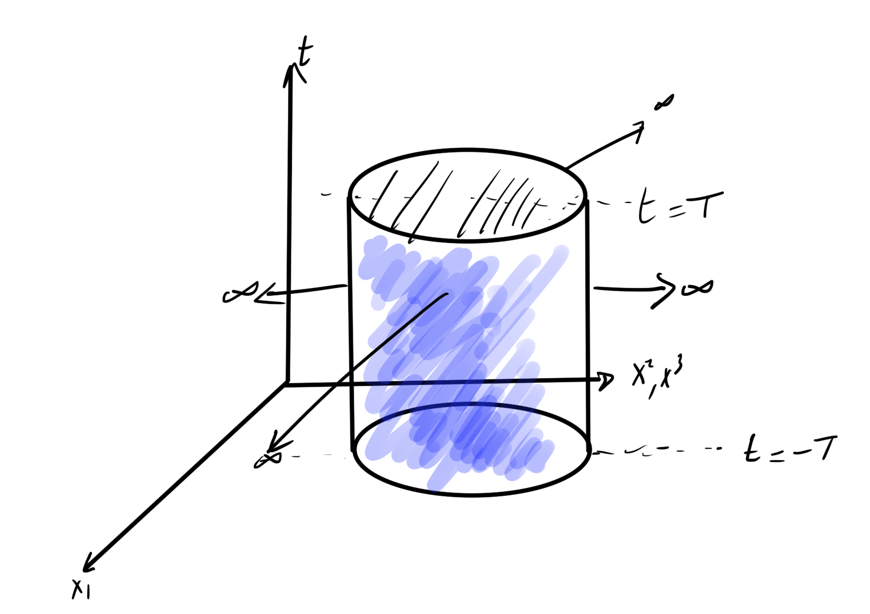
Classical scalar theory

For \( d > 2 \) let’s look at
\begin{equation}\label{eqn:qftLecture8:940}
S =
\int d^d x \lr{
\inv{2} \partial^\mu \phi \partial_\mu \phi – \frac{m^2}{2} \phi^2 – \lambda \phi^{d-2}
}
\end{equation}

Take \( m^2, \lambda \rightarrow 0 \), the free massless scalar field.

We have a shift symmetry in this case since \( \phi(x) \rightarrow \phi(x) + \text{constant} \).
The current is just
\begin{equation}\label{eqn:qftLecture8:960}
\begin{aligned}
j^\mu
&= \PD{(\partial_\mu \phi)}{\phi} \delta \phi – J^\mu \\
&= \PD{(\partial_\mu \phi)}{\phi} \delta \phi \\
&= \text{constant} \times \partial^\mu \phi \\
&= \partial^\mu \phi,
\end{aligned}
\end{equation}
where the constant factor has been set to one.
This current is clearly conserved since \( \partial_\mu J^\mu = \partial_\mu \partial^\mu \phi = 0\) (the equation of motion).

These are called “Goldstein Bosons”.

With \( m = \lambda = 0, d = 4 \) we have

NOTE: We did this in class differently with \( d \ne 4, m, \lambda \ne 0\), and then switched to \( m = \lambda = 0, d = 4\), which was confusing. I’ve reworked my notes to \( d = 4 \) like the supplemental handout that did the same.

\begin{equation}\label{eqn:qftLecture8:980}
S =
\int d^4 x \lr{
\inv{2} \partial^\mu \phi \partial_\mu \phi
}
\end{equation}
Here we have a scale or dilatation invariance
\begin{equation}\label{eqn:qftLecture8:1000}
x \rightarrow x’ = e^{\lambda} x,
\end{equation}
\begin{equation}\label{eqn:qftLecture8:1020}
\phi(x) \rightarrow \phi'(x’) = e^{-\lambda} \phi,
\end{equation}
\begin{equation}\label{eqn:qftLecture8:1040}
d^4 x \rightarrow d^4 x’ = e^{4\lambda} d^4 x,
\end{equation}

The partials transform as
\begin{equation}\label{eqn:qftLecture8:1400}
\partial^\mu \rightarrow
\PD{x’_\mu}{}
=
\PD{x’_\mu}{x_\mu}
\PD{x_\mu}{}
=
e^{-\lambda}
\PD{x_\mu}{}
\end{equation}

so the partial of the field transforms as
\begin{equation}\label{eqn:qftLecture8:1420}
\partial^\mu \phi(x) \rightarrow \PD{x’_\mu}{\phi'(x’)} = e^{-2\lambda} \partial^\mu \phi(x),
\end{equation}
and finally
\begin{equation}\label{eqn:qftLecture8:1060}
(\partial_\mu \phi)^2 \rightarrow e^{-4\lambda} \lr{ \partial_\mu \phi(x) }^2.
\end{equation}

With a \( -4 \lambda \) power in the transformed quadratic term, and \( 4 \lambda \) in the volume element, we see that the action is invariant.

To find Noether current, we need to vary the field and it’s derivatives
\begin{equation}\label{eqn:qftLecture8:1100}
\begin{aligned}
\delta_\lambda \phi
&= \phi'(x) – \phi(x) \\
&= \phi'(e^{-\lambda} x’) – \phi(x) \\
&\approx \phi'(x’ -\lambda x’) – \phi(x) \\
&\approx \phi'(x’) – \lambda {x’}^\alpha \partial_\alpha \phi'(x’) – \phi(x) \\
&\approx (1 – \lambda) \phi(x) – \lambda {x’}^\alpha \partial_\alpha \phi'(x’) – \phi(x) \\
&= – \lambda(1 + x^\alpha \partial_\alpha ) \phi,
\end{aligned}
\end{equation}
where the last step assumes that \( x’ \rightarrow x, \phi’ \rightarrow \phi \), effectively weeding out any terms that are quadratic or higher in \( \lambda \).

Now we need the variation of the derivatives of \( \phi \)
\begin{equation}\label{eqn:qftLecture8:1440}
\delta \partial_\mu \phi(x)
=
\partial_\mu’ \phi'(x) – \partial_\mu \phi(x),
\end{equation}
By \ref{eqn:qftLecture8:1420}
\begin{equation}\label{eqn:qftLecture8:1460}
\begin{aligned}
\partial_\mu’ \phi'(x’)
&=
e^{-2\lambda} \partial_\mu \phi(x) \\
&=
e^{-2\lambda} \partial_\mu \phi(e^{-\lambda} x’) \\
&\approx
e^{-2\lambda} \partial_\mu
\lr{
\phi(x’) – \lambda {x’}^\alpha \partial_\alpha \phi(x’)
} \\
&\approx
\lr{
1 – 2 \lambda
}
\partial_\mu
\lr{
\phi(x’) – \lambda {x’}^\alpha \partial_\alpha \phi(x’)
},
\end{aligned}
\end{equation}
so
\begin{equation}\label{eqn:qftLecture8:1480}
\begin{aligned}
\delta \partial_\mu \phi
&=
– \lambda {x}^\alpha \partial_\alpha \partial_\mu \phi(x)
– 2 \lambda \partial_\mu \phi(x) + O(\lambda^2) \\
&=
– \lambda \lr{
{x}^\alpha \partial_\alpha + 2
}
\partial_\mu \phi(x).
\end{aligned}
\end{equation}

\begin{equation}\label{eqn:qftLecture8:1200}
\begin{aligned}
\delta \LL
&=
(\partial^\mu \phi) \delta (\partial_\mu \phi) \\
&= – \lambda \lr{ 2
\partial_\mu \phi
+ x^\alpha \partial_\alpha
\partial_\mu \phi
}
\partial^\mu \phi,
\end{aligned}
\end{equation}
or
\begin{equation}\label{eqn:qftLecture8:1500}
\begin{aligned}
\frac{\delta \LL }{-\lambda}
&=
4 \LL + x^\alpha \lr{ \partial_\alpha \partial_\mu \phi } \partial^\mu \phi \\
&=
4 \LL + x^\alpha \partial_\alpha \lr{ \LL } \\
&=
{4 \LL} + \partial_\alpha \lr{ x^\alpha \LL } – {\LL \partial_\alpha x^\alpha} \\
&=
\partial_\alpha \lr{ x^\alpha \LL }.
\end{aligned}
\end{equation}
The variation in the Lagrangian density is thus
\begin{equation}\label{eqn:qftLecture8:1520}
\delta \LL = \partial_\mu J^\mu_\lambda = \partial_\mu \lr{ -\lambda x^\mu \LL },
\end{equation}
and the current is
\begin{equation}\label{eqn:qftLecture8:1540}
J^\mu_\lambda = -\lambda x^\mu \LL.
\end{equation}

The Noether current is
\begin{equation}\label{eqn:qftLecture8:1240}
\begin{aligned}
j^\mu
&= \PD{(\partial_\mu \phi)}{\LL} \delta \phi – J^\mu \\
&= -\partial^\mu \phi \lr{ 1 + x^\nu \partial_\nu } \phi + \inv{2} x^\mu \partial_\nu \phi \partial^\nu \phi,
\end{aligned}
\end{equation}
or after flipping signs
\begin{equation}\label{eqn:qftLecture8:1280}
\begin{aligned}
j^\mu_{\text{dil}}
&= \partial^\mu \phi \lr{ 1 + x^\nu \partial_\nu } \phi – \inv{2} x^\mu
\partial_\nu \phi \partial^\nu \phi \\
&= x_\nu \lr{ \partial^\mu \phi \partial^\nu \phi – \inv{2} {\delta^{\nu}}_\mu \partial_\lambda \phi \partial^\lambda \phi }
+ \inv{2} \partial^\mu (\phi^2),
\end{aligned}
\end{equation}

\begin{equation}\label{eqn:qftLecture8:1300}
j^\mu_{\text{dil}} = -x_\nu T^{\nu \mu} + \inv{2} \partial^\mu (\phi^2),
\end{equation}

The current and \( T^{\mu\nu} \) can both be redefined \( j^{\mu’} = j^\mu + \partial_\nu C^{\nu\mu} \) adding an antisymmetric \( C^{\mu\nu} = -C^{\nu\mu} \)

\begin{equation}\label{eqn:qftLecture8:1320}
j^\mu_{\text{dil conformal}} = – x_\nu T^{\nu\mu}_{\text{conformal}}
\end{equation}

\begin{equation}\label{eqn:qftLecture8:1340}
\partial_\mu
j^\mu_{\text{dil conformal}} = – {{T_{\text{conformal}}}^\mu}_\mu
\end{equation}

consequence: \( 0 = T^{00} – T^{11} – T^{22} – T^{33} \), which is essentially
\begin{equation}\label{eqn:qftLecture8:1360}
0 = \rho – 3 p = 0.
\end{equation}

Energy-momentum tensor for a scalar field

January 5, 2016 phy2403 , ,

[Click here for a PDF of this post with nicer formatting]

It is claimed in [1] (3.2.1) that the momentum components of the energy-momentum tensor was found to be

\begin{equation}\label{eqn:noetherCurrentScalarField:20}
\Be_n \int d^3 x T^{0 n} = \int d^3 k \Bk a_k^\dagger a_k.
\end{equation}

I don’t see this result anywhere, so let’s calculate it.

First, from the Noether current for the scalar field Lagrangian in question, what is the energy-momentum tensor explicitly?

\begin{equation}\label{eqn:noetherCurrentScalarField:40}
\begin{aligned}
T^{\mu \nu}
&= \Pi^\mu \partial^\nu \phi – g^{\mu \nu} \LL \\
&= \Pi^\mu \partial^\nu \phi – g^{\mu \nu} \inv{2} \lr{ \partial_\alpha \phi \partial^\alpha \phi – \mu^2 \phi^2 } \\
&= \Pi^\mu \Pi^\nu – g^{\mu \nu} \inv{2} \lr{ \Pi_\alpha \Pi^\alpha – \mu^2 \phi^2 } \\
&= \Pi^\mu \Pi^\nu – \inv{2} g^{\mu \nu} g_{\alpha\beta} \Pi^\beta \Pi^\alpha + \inv{2} g^{\mu \nu} \mu^2 \phi^2.
\end{aligned}
\end{equation}

Consider some special cases for the indexes. For \( \mu = \nu = 0 \), the result is the Hamiltonian density

\begin{equation}\label{eqn:noetherCurrentScalarField:200}
\begin{aligned}
T^{00}
&= \Pi^0 \Pi^0 – \inv{2} g^{0 0} \Pi_\alpha \Pi^\alpha + \inv{2} g^{0 0} \mu^2 \phi^2 \\
&= \Pi^0 \Pi^0 – \inv{2} \Pi_\alpha \Pi^\alpha + \inv{2} \mu^2 \phi^2 \\
&= \inv{2} \Pi^0 \Pi^0 – \inv{2} \Pi_n \Pi^n + \inv{2} \mu^2 \phi^2 \\
&= \inv{2} \Pi^2 + \inv{2} (\spacegrad \phi)^2 + \inv{2} \mu^2 \phi^2,
\end{aligned}
\end{equation}

where \( \Pi^2 = (\partial_0 \phi)^2 \ne \partial^2 \phi \). For any \( \mu \ne \nu \) the off diagonal metric elements are zero, leaving just
\begin{equation}\label{eqn:noetherCurrentScalarField:220}
T^{\mu\nu} = \Pi^\mu \Pi^\nu.
\end{equation}

Finally, when \( n \ne 0 \), the remaining diagonal terms are
\begin{equation}\label{eqn:noetherCurrentScalarField:240}
\begin{aligned}
T^{nn}
&= \Pi^n \Pi^n – \inv{2} g^{n n} \Pi_\alpha \Pi^\alpha + \inv{2} g^{n n} n^2 \phi^2 \\
&= \Pi^n \Pi^n + \inv{2} \Pi_\alpha \Pi^\alpha – \inv{2} \mu^2 \phi^2 \\
&= \inv{2} \Pi^2 + \Pi^n \Pi^n – \inv{2} \Pi^m \Pi^m – \inv{2} \mu^2 \phi^2 \\
&= \inv{2} \Pi^2 + \inv{2} \Pi^n \Pi^n – \inv{2} \sum_{m\ne n,0} \Pi^m \Pi^m – \inv{2} \mu^2 \phi^2 \\
&= \inv{2} \sum_{m = n,0} \Pi^m \Pi^m – \inv{2} \sum_{m\ne n,0} \Pi^m \Pi^m – \inv{2} \mu^2 \phi^2.
\end{aligned}
\end{equation}

The canonical momenta are

\begin{equation}\label{eqn:noetherCurrentScalarField:60}
\Pi^\mu
=
\partial^\mu
\int \frac{d^3 k}{(2\pi)^{3/2} \sqrt{ 2 \omega_k }} \lr{ a_k e^{-i k \cdot x} + a_k^\dagger e^{i k \cdot x} },
\end{equation}

but
\begin{equation}\label{eqn:noetherCurrentScalarField:80}
\begin{aligned}
\partial^\mu e^{i k \cdot x}
&=
\partial^\mu \exp\lr{ i k^\alpha x_\alpha } \\
&=
i k^\mu \exp\lr{ i k \cdot x },
\end{aligned}
\end{equation}

so
\begin{equation}\label{eqn:noetherCurrentScalarField:100}
\begin{aligned}
\Pi^\mu
&=
i
\int \frac{d^3 k k^\mu}{(2\pi)^{3/2} \sqrt{ 2 \omega_k }} \lr{ – a_k e^{-i k \cdot x} + a_k^\dagger e^{i k \cdot x} } \\
&=
i
\int \frac{d^3 k k^\mu}{(2\pi)^{3/2} \sqrt{ 2 \omega_k }} \lr{ – a_k e^{-i \omega_k t + \Bk \cdot \Bx} + a_k^\dagger e^{i \omega_k t – i \Bk \cdot \Bx} }.
\end{aligned}
\end{equation}

This gives
\begin{equation}\label{eqn:noetherCurrentScalarField:120}
\begin{aligned}
\int d^3 x \Pi^\mu \Pi^\nu
&=
-\inv{2} \int d^3 x \inv{(2\pi)^3}
\int d^3 k d^3 j \frac{k^\mu j^\nu}{\sqrt{\omega_k \omega_j}}
\lr{ – a_k e^{-i \omega_k t + \Bk \cdot \Bx} + a_k^\dagger e^{i \omega_k t – i \Bk \cdot \Bx} }
\lr{ – a_j e^{-i \omega_j t + \Bj \cdot \Bx} + a_j^\dagger e^{i \omega_j t – i \Bj \cdot \Bx} } \\
&=
-\inv{2} \int d^3 x \inv{(2\pi)^3}
\int d^3 k d^3 j \frac{k^\mu j^\nu}{\sqrt{\omega_k \omega_j}}
\lr{
a_k a_j e^{-i (\omega_j + \omega_k) t + (\Bj + \Bk) \cdot \Bx}
– a_k a_j^\dagger e^{i (\omega_j – \omega_k) t – i (\Bj -\Bk) \cdot \Bx}
– a_k^\dagger a_j e^{-i (\omega_j -\omega_k) t – (\Bk – \Bj) \cdot \Bx}
+ a_k^\dagger a_j^\dagger e^{i (\omega_j + \omega_k) t – i (\Bj + \Bk) \cdot \Bx}
} \\
&=
-\inv{2}
\int d^3 k d^3 j \frac{k^\mu j^\nu}{\sqrt{\omega_k \omega_j}}
\lr{
a_k a_j e^{-i (\omega_j + \omega_k) t } \delta^3(\Bj + \Bk)
– a_k a_j^\dagger e^{i (\omega_j – \omega_k) t } \delta^3(\Bj -\Bk)
– a_k^\dagger a_j e^{-i (\omega_j -\omega_k) t } \delta^3 (\Bk – \Bj)
+ a_k^\dagger a_j^\dagger e^{i (\omega_j + \omega_k) t } \delta^3 (\Bj + \Bk)
}.
\end{aligned}
\end{equation}

There are two cases here to consider. The first is \( \nu = 0 \), for which

\begin{equation}\label{eqn:noetherCurrentScalarField:140}
\int d^3 x \Pi^\mu \Pi^0
=
-\inv{2}
\int d^3 k k^\mu
\lr{
a_k a_{-k} e^{-2 i \omega_k t }
– a_k a_k^\dagger
– a_k^\dagger a_k
+ a_k^\dagger a_{-k}^\dagger e^{2 i \omega_k t }
}.
\end{equation}

For \( \nu \ne 0 \)

\begin{equation}\label{eqn:noetherCurrentScalarField:160}
\begin{aligned}
\int d^3 x \Pi^\mu \Pi^\nu
&=
-\inv{2}
\int d^3 k \frac{k^\mu k^\nu}{\omega_k}
\lr{
– a_k a_{-k} e^{- 2 i \omega_k t }
– a_k a_k^\dagger
– a_k^\dagger a_k
– a_k^\dagger a_{-k}^\dagger e^{ 2 i \omega_k t }
} \\
&=
\inv{2}
\int d^3 k \frac{k^\mu k^\nu}{\omega_k}
\lr{
a_k a_{-k} e^{- 2 i \omega_k t }
+ a_k a_k^\dagger
+ a_k^\dagger a_k
+ a_k^\dagger a_{-k}^\dagger e^{ 2 i \omega_k t }
}.
\end{aligned}
\end{equation}

Here’s a summary of these products

\begin{equation}\label{eqn:noetherCurrentScalarField:300}
\int d^3 x \Pi^0 \Pi^0
=
-\inv{2}
\int d^3 k \omega_k
\lr{
a_k a_{-k} e^{-2 i \omega_k t }
– a_k a_k^\dagger
– a_k^\dagger a_k
+ a_k^\dagger a_{-k}^\dagger e^{2 i \omega_k t }
},
\end{equation}
\begin{equation}\label{eqn:noetherCurrentScalarField:280}
\int d^3 x \Pi^n \Pi^0
= \int d^3 x \Pi^0 \Pi^n
=
-\inv{2}
\int d^3 k k^n
\lr{
a_k a_{-k} e^{-2 i \omega_k t }
– a_k a_k^\dagger
– a_k^\dagger a_k
+ a_k^\dagger a_{-k}^\dagger e^{2 i \omega_k t }
},
\end{equation}
\begin{equation}\label{eqn:noetherCurrentScalarField:340}
\int d^3 x \Pi^m \Pi^n
=
\inv{2}
\int d^3 k \frac{k^m k^n}{\omega_k}
\lr{
a_k a_{-k} e^{- 2 i \omega_k t }
+ a_k a_k^\dagger
+ a_k^\dagger a_k
+ a_k^\dagger a_{-k}^\dagger e^{ 2 i \omega_k t }
}.
\end{equation}

For the mass term it was previously found that

\begin{equation}\label{eqn:noetherCurrentScalarField:180}
\inv{2} \int d^3 x \mu^2 \phi^2
=
\frac{\mu^2}{4}
\int
d^3 k
\inv{ \omega_k }
\lr{
a_{-k} a_k e^{- 2 i \omega_k t }
+a_{-k}^\dagger a_k^\dagger e^{2 i \omega_k t }
+a_k a_k^\dagger
+a_k^\dagger a_k
}.
\end{equation}

The Hamiltonian component has been previously calculated, and resolves to

\begin{equation}\label{eqn:noetherCurrentScalarField:360}
\int d^3 x T^{00}
=
\inv{2}
\int d^3 k
\omega_k
\lr{
a_k a_k^\dagger
+ a_k^\dagger a_k
}.
\end{equation}

The other diagonal components, for \( r \ne s \ne t \) are
\begin{equation}\label{eqn:noetherCurrentScalarField:380}
\begin{aligned}
\int d^3 x T^{rr}
&=
\int d^3 x
\lr{
\inv{2} \sum_{m = r,0} \Pi^m \Pi^m – \inv{2} \sum_{m = s,t} \Pi^m \Pi^m – \inv{2} \mu^2 \phi^2
} \\
&=
\inv{4}
\int d^3 k \frac{(k^r)^2 – (k^s)^2 – (k^t)^2 – \mu^2}{\omega_k}
\lr{
a_k a_{-k} e^{- 2 i \omega_k t }
+ a_k a_k^\dagger
+ a_k^\dagger a_k
+ a_k^\dagger a_{-k}^\dagger e^{ 2 i \omega_k t }
}
-\inv{4}
\int d^3 k \omega_k
\lr{
a_k a_{-k} e^{-2 i \omega_k t }
– a_k a_k^\dagger
– a_k^\dagger a_k
+ a_k^\dagger a_{-k}^\dagger e^{2 i \omega_k t }
} \\
&=
\inv{4}
\int d^3 k \frac{(k^r)^2 – (k^s)^2 – (k^t)^2 – \mu^2 – \omega_k^2}{\omega_k}
\lr{
a_k a_{-k} e^{- 2 i \omega_k t }
+ a_k^\dagger a_{-k}^\dagger e^{ 2 i \omega_k t }
}
+
\inv{4}
\int d^3 k \frac{(k^r)^2 – (k^s)^2 – (k^t)^2 – \mu^2 + \omega_k^2}{\omega_k}
\lr{
a_k a_k^\dagger
+ a_k^\dagger a_k
} \\
&=
\inv{2}
\int d^3 k \frac{ (k^r)^2 – \omega_k^2}{\omega_k}
\lr{
a_k a_{-k} e^{- 2 i \omega_k t }
+ a_k^\dagger a_{-k}^\dagger e^{ 2 i \omega_k t }
}
+
\inv{2}
\int d^3 k \frac{ (k^r)^2}{\omega_k}
\lr{
a_k a_k^\dagger
+ a_k^\dagger a_k
}.
\end{aligned}
\end{equation}

This doesn’t have the nice cancelation that killed the time dependent terms in the Hamiltonian. Such cancellation also doesn’t appear in the off diagonal energy-momentum tensor components, which are

\begin{equation}\label{eqn:noetherCurrentScalarField:400}
\begin{aligned}
\int d^3 x T^{n 0}
&=
\int d^3 x T^{n 0} \\
&=
-\inv{2}
\int d^3 k k^n
\lr{
a_k a_{-k} e^{-2 i \omega_k t }
– a_k a_k^\dagger
– a_k^\dagger a_k
+ a_k^\dagger a_{-k}^\dagger e^{2 i \omega_k t }
},
\end{aligned}
\end{equation}

and for \( m \ne n \ne 0 \)
\begin{equation}\label{eqn:noetherCurrentScalarField:420}
\int d^3 x T^{m n}
=
\inv{2}
\int d^3 k \frac{k^m k^n}{\omega_k}
\lr{
a_k a_{-k} e^{- 2 i \omega_k t }
+ a_k a_k^\dagger
+ a_k^\dagger a_k
+ a_k^\dagger a_{-k}^\dagger e^{ 2 i \omega_k t }
}.
\end{equation}

The \ref{eqn:noetherCurrentScalarField:400} result has time dependence that the stated result does not (but is linear in \( \Bk \) as desired)? Did I miss something?

References

[1] Michael Luke. PHY2403F Lecture Notes: Quantum Field Theory, 2015. URL https://piazza.com/utoronto.ca/fall2015/phy2403f/resources. [Online; accessed 02-Jan-2016].

Energy momentum conservation with magnetic sources

February 20, 2015 ece1229 , , , , , , , , , , , , , , ,

[Click here for a PDF of this post with nicer formatting]

Maxwell’s equations with magnetic sources

The form of Maxwell’s equations to be used here are expressed in terms of \( \boldsymbol{\mathcal{E}} \) and \( \boldsymbol{\mathcal{H}} \), assume linear media, and do not assume a phasor representation

\begin{equation}\label{eqn:energyMomentumWithMagneticSources:120}
\spacegrad \cross \boldsymbol{\mathcal{E}} = – \boldsymbol{\mathcal{M}} – \mu_0 \PD{t}{\boldsymbol{\mathcal{H}}}
\end{equation}
\begin{equation}\label{eqn:energyMomentumWithMagneticSources:140}
\spacegrad \cross \boldsymbol{\mathcal{H}} = \boldsymbol{\mathcal{J}} + \epsilon_0 \PD{t}{\boldsymbol{\mathcal{E}}}
\end{equation}
\begin{equation}\label{eqn:energyMomentumWithMagneticSources:160}
\spacegrad \cdot \boldsymbol{\mathcal{E}} = \rho/\epsilon_0
\end{equation}
\begin{equation}\label{eqn:energyMomentumWithMagneticSources:180}
\spacegrad \cdot \boldsymbol{\mathcal{H}} = \rho_m/\mu_0.
\end{equation}

Energy momentum conservation

With magnetic sources the Poynting and energy conservation relationship has to be adjusted slightly. Let’s derive that result, starting with the divergence of the Poynting vector

\begin{equation}\label{eqn:energyMomentumWithMagneticSources:20}
\begin{aligned}
\spacegrad \cdot \lr{ \boldsymbol{\mathcal{E}} \cross \boldsymbol{\mathcal{H}} }
&=
\boldsymbol{\mathcal{H}} \cdot \lr{ \spacegrad \cross \boldsymbol{\mathcal{E}} }
-\boldsymbol{\mathcal{E}} \cdot \lr{ \spacegrad \cross \boldsymbol{\mathcal{H}} } \\
&=
-\boldsymbol{\mathcal{H}} \cdot \lr{ \mu_0 \partial_t \boldsymbol{\mathcal{H}} + \boldsymbol{\mathcal{M}} }
-\boldsymbol{\mathcal{E}} \cdot \lr{ \boldsymbol{\mathcal{J}} + \epsilon_0 \partial_t \boldsymbol{\mathcal{E}} } \\
&=
– \mu_0 \boldsymbol{\mathcal{H}} \cdot \partial_t \boldsymbol{\mathcal{H}} – \boldsymbol{\mathcal{H}} \cdot \boldsymbol{\mathcal{M}}
– \epsilon_0 \boldsymbol{\mathcal{E}} \cdot \partial_t \boldsymbol{\mathcal{E}} – \boldsymbol{\mathcal{E}} \cdot \boldsymbol{\mathcal{J}},
\end{aligned}
\end{equation}

or

\begin{equation}\label{eqn:energyMomentumWithMagneticSources:40}
\boxed{
\inv{2} \PD{t}{} \lr{ \epsilon_0 \boldsymbol{\mathcal{E}}^2 + \mu_0 \boldsymbol{\mathcal{H}}^2 }
+
\spacegrad \cdot \lr{ \boldsymbol{\mathcal{E}} \cross \boldsymbol{\mathcal{H}} }
=
– \boldsymbol{\mathcal{H}} \cdot \boldsymbol{\mathcal{M}}
– \boldsymbol{\mathcal{E}} \cdot \boldsymbol{\mathcal{J}}.
}
\end{equation}

The usual relationship is only modified by one additional term. Recall from electrodynamics [2] that \ref{eqn:energyMomentumWithMagneticSources:40} (when the magnetic current density \( \boldsymbol{\mathcal{M}} \) is omitted) is just one of four components of the energy momentum conservation equation

\begin{equation}\label{eqn:energyMomentumWithMagneticSources:80}
\partial_\mu T^{\mu \nu} = – \inv{c} F^{\nu \lambda} j_\lambda.
\end{equation}

Note that \ref{eqn:energyMomentumWithMagneticSources:80} was likely not in SI units. The next task is to generalize this classical relationship to incorporate the magnetic sources used in antenna theory. With an eye towards the relativistic nature of the energy momentum tensor, it is natural to assume that the remainder of the energy momentum tensor conservation relation can be found by taking the time derivatives of the Poynting vector.

\begin{equation}\label{eqn:energyMomentumWithMagneticSources:200}
\PD{t}{} \lr{ \boldsymbol{\mathcal{E}} \cross \boldsymbol{\mathcal{H}} }
=
\PD{t}{\boldsymbol{\mathcal{E}}} \cross \boldsymbol{\mathcal{H}}
+ \boldsymbol{\mathcal{E}} \cross \PD{t}{\boldsymbol{\mathcal{H}} }
=
\inv{\epsilon_0}
\lr{ \spacegrad \cross \boldsymbol{\mathcal{H}} – \boldsymbol{\mathcal{J}} } \cross \boldsymbol{\mathcal{H}}
+
\inv{\mu_0}
\boldsymbol{\mathcal{E}} \cross
\lr{

\spacegrad \cross \boldsymbol{\mathcal{E}} – \boldsymbol{\mathcal{M}} },
\end{equation}

or

\begin{equation}\label{eqn:energyMomentumWithMagneticSources:220}
\inv{c^2} \PD{t}{} \lr{ \boldsymbol{\mathcal{E}} \cross \boldsymbol{\mathcal{H}} }
+
\mu_0 \boldsymbol{\mathcal{J}} \cross \boldsymbol{\mathcal{H}}
+\epsilon_0
\boldsymbol{\mathcal{E}} \cross \boldsymbol{\mathcal{M}}
=
-\mu_0 \boldsymbol{\mathcal{H}} \cross \lr{ \spacegrad \cross \boldsymbol{\mathcal{H}} }
– \epsilon_0 \boldsymbol{\mathcal{E}} \cross \lr{ \spacegrad \cross \boldsymbol{\mathcal{E}} }.
\end{equation}

The \( \mu_0 \boldsymbol{\mathcal{J}} \cross \boldsymbol{\mathcal{H}} = \boldsymbol{\mathcal{J}} \cross \BB \) is a portion of the Lorentz force equation in its density form. To put \ref{eqn:energyMomentumWithMagneticSources:220} into the desired form, the remainder of the Lorentz force force equation \( \rho \boldsymbol{\mathcal{E}} = \epsilon_0 \boldsymbol{\mathcal{E}} \spacegrad \cdot \boldsymbol{\mathcal{E}} \) must be added to both sides. To extend the magnetic current term to its full dual (magnetic) Lorentz force structure, the quantity to add to both sides is \( \rho_m \boldsymbol{\mathcal{H}} = \mu_0 \boldsymbol{\mathcal{H}} \spacegrad \cdot \boldsymbol{\mathcal{H}} \). Performing these manipulations gives

\begin{equation}\label{eqn:energyMomentumWithMagneticSources:240}
\inv{c^2} \PD{t}{} \lr{ \boldsymbol{\mathcal{E}} \cross \boldsymbol{\mathcal{H}} }
+
\rho \BE + \mu_0 \boldsymbol{\mathcal{J}} \cross \boldsymbol{\mathcal{H}}
+ \rho_m \boldsymbol{\mathcal{H}}
+ \epsilon_0 \boldsymbol{\mathcal{E}} \cross \boldsymbol{\mathcal{M}}
=
\mu_0
\lr{
\boldsymbol{\mathcal{H}} \spacegrad \cdot \boldsymbol{\mathcal{H}}
-\boldsymbol{\mathcal{H}} \cross \lr{ \spacegrad \cross \boldsymbol{\mathcal{H}} }
}
+ \epsilon_0
\lr{
\boldsymbol{\mathcal{E}} \spacegrad \cdot \boldsymbol{\mathcal{E}}

\boldsymbol{\mathcal{E}} \cross \lr{ \spacegrad \cross \boldsymbol{\mathcal{E}} }
}.
\end{equation}

It seems slightly surprising the sign of the magnetic equivalent of the Lorentz force terms have an alternation of sign. This is, however, consistent with the duality transformations outlined in ([1] table 3.2)

\begin{equation}\label{eqn:energyMomentumWithMagneticSources:280}
\rho \rightarrow \rho_m
\end{equation}
\begin{equation}\label{eqn:energyMomentumWithMagneticSources:300}
\boldsymbol{\mathcal{J}} \rightarrow \boldsymbol{\mathcal{M}}
\end{equation}
\begin{equation}\label{eqn:energyMomentumWithMagneticSources:320}
\mu_0 \rightarrow \epsilon_0
\end{equation}
\begin{equation}\label{eqn:energyMomentumWithMagneticSources:340}
\boldsymbol{\mathcal{E}} \rightarrow \boldsymbol{\mathcal{H}}
\end{equation}
\begin{equation}\label{eqn:energyMomentumWithMagneticSources:360}
\boldsymbol{\mathcal{H}} \rightarrow -\boldsymbol{\mathcal{E}},
\end{equation}

for

\begin{equation}\label{eqn:energyMomentumWithMagneticSources:380}
\rho \BE + \mu_0 \boldsymbol{\mathcal{J}} \cross \boldsymbol{\mathcal{H}}
\rightarrow
\rho_m \BH + \epsilon_0 \boldsymbol{\mathcal{M}} \cross \lr{ -\boldsymbol{\mathcal{E}}}
=
\rho_m \BH + \epsilon_0 \boldsymbol{\mathcal{E}} \cross \boldsymbol{\mathcal{M}}.
\end{equation}

Comfortable that the LHS has the desired structure, the RHS can expressed as a divergence. Just expanding one of the differences of vector products on the RHS does not obviously show that this is possible, for example

\begin{equation}\label{eqn:energyMomentumWithMagneticSources:400}
\begin{aligned}
\Be_a \cdot
\lr{
\boldsymbol{\mathcal{E}} \spacegrad \cdot \boldsymbol{\mathcal{E}}

\boldsymbol{\mathcal{E}} \cross \lr{ \spacegrad \cross \boldsymbol{\mathcal{E}} }
}
&=
E_a \partial_b E_b

\epsilon_{a b c} E_b \epsilon_{c r s} \partial_r E_s \\
&=
E_a \partial_b E_b

\delta_{a b}^{[r s]} E_b \partial_r E_s \\
&=
E_a \partial_b E_b

E_b \lr{
\partial_a E_b
-\partial_b E_a
} \\
&=
E_a \partial_b E_b
– E_b \partial_a E_b
+ E_b \partial_b E_a.
\end{aligned}
\end{equation}

This happens to equal

\begin{equation}\label{eqn:energyMomentumWithMagneticSources:420}
\begin{aligned}
\spacegrad \cdot \lr{ \lr{E_a E_b – \inv{2} \delta_{a b} \boldsymbol{\mathcal{E}}^2 } \Be_b }
&=
\partial_b
\lr{E_a E_b – \inv{2} \delta_{a b} \boldsymbol{\mathcal{E}}^2 } \\
&=
E_b \partial_b E_a
+ E_a \partial_b E_b

\inv{2} \delta_{a b} 2 E_c \partial_b E_c \\
i&=
E_b \partial_b E_a
+ E_a \partial_b E_b
– E_b \partial_a E_b.
\end{aligned}
\end{equation}

This allows a final formulation of the remaining energy momentum conservation equation in its divergence form. Let

\begin{equation}\label{eqn:energyMomentumWithMagneticSources:440}
T^{a b} =
\epsilon_0 \lr{ E_a E_b – \inv{2} \delta_{a b} \boldsymbol{\mathcal{E}}^2 }
+ \mu_0 \lr{ H_a H_b – \inv{2} \delta_{a b} \boldsymbol{\mathcal{H}}^2 },
\end{equation}

so that the remaining energy momentum conservation equation, extended to both electric and magnetic sources, is

\begin{equation}\label{eqn:energyMomentumWithMagneticSources:460}
\boxed{
\inv{c^2} \PD{t}{} \lr{ \boldsymbol{\mathcal{E}} \cross \boldsymbol{\mathcal{H}} }
+
\rho \BE + \mu_0 \boldsymbol{\mathcal{J}} \cross \boldsymbol{\mathcal{H}}
+ \rho_m \boldsymbol{\mathcal{H}}
+ \epsilon_0 \boldsymbol{\mathcal{E}} \cross \boldsymbol{\mathcal{M}}
=
\Be_a \spacegrad \cdot \lr{ T^{a b} \Be_b }.
}
\end{equation}

On the LHS we have the rate of change of momentum density, the electric Lorentz force density terms, the dual (magnetic) Lorentz force density terms, and on the RHS the the momentum flux terms.

References

[1] Constantine A Balanis. Antenna theory: analysis and design. John Wiley \& Sons, 3rd edition, 2005.

[2] Peeter Joot. Relativistic Electrodynamics., chapter {Energy Momentum Tensor.} peeterjoot.com, 2011. URL https://peeterjoot.com/archives/math2011/phy450.pdf. [Online; accessed 18-February-2015].