[Click here for a PDF version of this post]
Motivation
Maverick posed the following question on the bivector discord
“I saw your blog post on curvilinear coordinates in geometric calculus. I saw your derivation of the volume of a sphere using this technique and decided for practice by doing a surface integral to calculate the area of sphere using the quantity $\partial{\theta} \wedge \partial{\phi}~ dA$ is there a way to integrate this without simply taking the magnitude of this quantity and then integrating or are we limited to only integrating quantities that are 1 dimensional like scalars and pseudoscalars”.
My initial response was that, sure, we should be able to compute bivector and trivector valued integrals. However, in retrospect, the reality is a bit more subtle.
We aren’t limited to using the magnitudes of the differential forms, but not all multivector integral are interesting.
In the original blog post, I must have computed the area of the circle using a bivector valued area element, or the volume of a sphere using a trivector valued volume element. However, if I did the volume that way, I probably cheated and computed 8 times the value of the first octant volume (which is positive), vs. the entire integral, which is zero. [EDIT: the original post, now linked above, has been corrected.]
Let’s compute the circular area and circumference, and the spherical volume and surface area using multivector valued integrals, and see where we end up having to resort to scalar integrals.
Circular example.
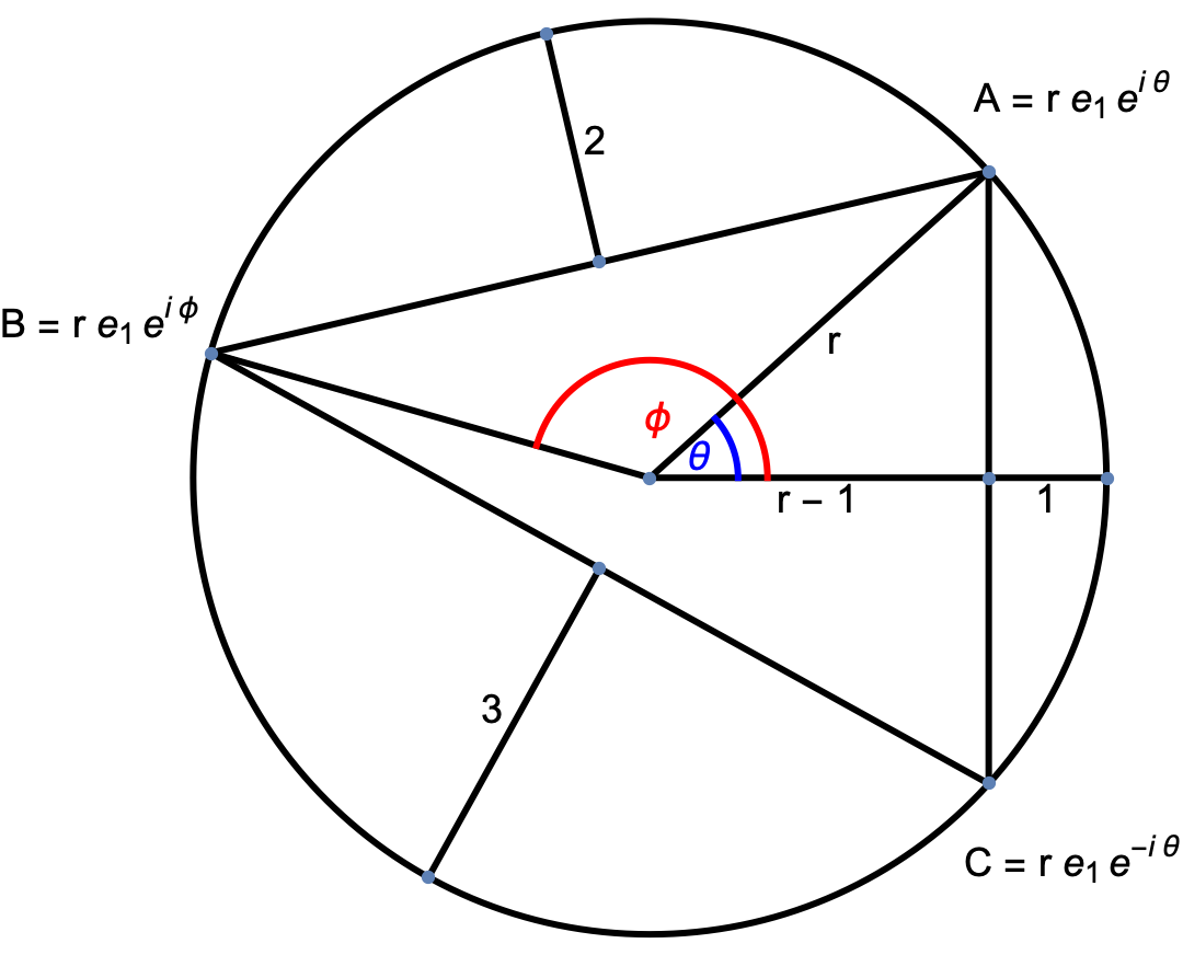
The polar parameterization of points in circular region is
\begin{equation}\label{eqn:circularAndSphericalAreaVolumeAndBoundaries:20}
\Bx = r \Be_1 e^{i\theta},
\end{equation}
where \( i = \Be_1 \Be_2 \).
Our differentials are
\begin{equation}\label{eqn:circularAndSphericalAreaVolumeAndBoundaries:40}
\begin{aligned}
d\Bx_r &= \Be_1 e^{i\theta} \,dr \\
d\Bx_\theta &= r \Be_2 e^{i\theta} \,d\theta.
\end{aligned}
\end{equation}
Our “volume” element, is a 2D pseudoscalar
\begin{equation}\label{eqn:circularAndSphericalAreaVolumeAndBoundaries:60}
\begin{aligned}
dA &= d\Bx_r \wedge d\Bx_\theta \\
&= r \gpgradetwo{ \Be_1 e^{i\theta} \Be_2 e^{i\theta} } \, dr d\theta \\
&= r \gpgradetwo{ \Be_1 \Be_2 e^{-i\theta} e^{i\theta} } \, dr d\theta \\
&= r i \, dr d\theta.
\end{aligned}
\end{equation}
This, as I probably pointed out in my previous blog post, can be integrated to find the area of the circle
\begin{equation}\label{eqn:circularAndSphericalAreaVolumeAndBoundaries:80}
\begin{aligned}
A &= \int_{r = 0}^R \int_{\theta = 0}^{2\pi} r i \, dr d\theta \\
&= \frac{R^2}{2} 2 \pi i \\
&= \pi R^2 i.
\end{aligned}
\end{equation}
However, we got lucky, as the two-form area element was strictly positive (i.e.: the Jacobean for a polar change of coordinates is strictly positive.)
However, we can’t find the circumference of a circle my integrating \( d\Bx_\theta \) around that circular path, because \( d\Bx_\theta \) has an orientation, and we will get zero (given the symmetry of the problem) if we integrate all the way around
\begin{equation}\label{eqn:circularAndSphericalAreaVolumeAndBoundaries:100}
\begin{aligned}
\int_{\theta = 0}^{2\pi} d\Bx_\theta &= \int_{\theta = 0}^{2\pi} r \Be_2 e^{i\theta} \,d\theta \\
&= r \Be_2 \evalrange{ \frac{e^{i\theta}}{i} }{0}{2\pi} \\
&= \frac{r \Be_2}{i} \times 0.
\end{aligned}
\end{equation}
If we want the circumference of a circle, we have to sum all the contributions of \( d\Bx_\theta \) that are colinear with \( \thetacap = \Be_2 e^{i\theta} \)
\begin{equation}\label{eqn:circularAndSphericalAreaVolumeAndBoundaries:120}
\begin{aligned}
C &= \int_{\theta = 0}^{2\pi} \thetacap \cdot \, d\Bx_\theta \\
&= \int_{\theta = 0}^{2\pi} \thetacap \cdot \lr{ r \thetacap \, d\theta } \\
&= 2 \pi r.
\end{aligned}
\end{equation}
This is a plain old boring scalar integral, because the vector valued path integral isn’t terribly interesting.
Spherical example.
For a spherical parameterization, our position vector is
\begin{equation}\label{eqn:circularAndSphericalAreaVolumeAndBoundaries:140}
\Bx = r \Be_1 e^{i \phi} \sin\theta + r \Be_3 \cos\theta,
\end{equation}
so the differentials are
\begin{equation}\label{eqn:circularAndSphericalAreaVolumeAndBoundaries:160}
\begin{aligned}
d\Bx_r &= \lr{ \Be_1 e^{i \phi} \sin\theta + \Be_3 \cos\theta } \,dr = \rcap \, dr \\
d\Bx_\theta &= \lr{ r \Be_1 e^{i \phi} \cos\theta – r \Be_3 \sin\theta }\, d\theta = r \thetacap \,d\theta \\
d\Bx_\phi &= r \Be_2 e^{i \phi} \sin\theta \, d\phi = r \sin\theta \phicap.
\end{aligned}
\end{equation}
The oriented area element on the surface of the sphere is
\begin{equation}\label{eqn:circularAndSphericalAreaVolumeAndBoundaries:180}
\begin{aligned}
dA &= d\Bx_\theta \wedge d\Bx_\phi \\
&= r^2 \gpgradetwo{ \lr{ \Be_1 e^{i \phi} \cos\theta – \Be_3 \sin\theta } \Be_2 e^{i \phi} \sin\theta } \,d\theta d\phi \\
&= r^2 \sin\theta \lr{ i \cos\theta – \Be_{32} e^{i \phi} \sin\theta } \,d\theta d\phi .
\end{aligned}
\end{equation}
Integrating this over the surface will give us zero, with the first integrand killed by the \( \theta \) integral, and the second by the \( \phi \) integral. As pointed out in the original question, we must integrate the absolute value of this two-form in order to find the surface area of the sphere, just as we had to integrate the absolute value of \( d\Bx_\theta \) for the circle to find the circumference.
Let’s perform that integration to verify that we get the expected result. We will first simplify our bivector valued oriented area element. Observe that \( dA \wedge \rcap = dA \rcap \propto I \), so \( dA \propto \rcap I \). We should be able to simplify our expression for \( dA \) by factoring out an \( \rcap \) term
\begin{equation}\label{eqn:circularAndSphericalAreaVolumeAndBoundaries:200}
\begin{aligned}
dA &= r^2 \sin\theta \lr{ \Be_{1233} \cos\theta – \Be_{1132} e^{i \phi} \sin\theta } \,d\theta d\phi \\
&= r^2 \sin\theta I \lr{ \Be_3 \cos\theta + \Be_1 e^{i \phi} \sin\theta } \,d\theta d\phi \\
&= r^2 \sin\theta I \rcap \,d\theta d\phi.
\end{aligned}
\end{equation}
The spherical scalar area is
\begin{equation}\label{eqn:circularAndSphericalAreaVolumeAndBoundaries:220}
\begin{aligned}
A
&= \int_{\theta = 0}^{\pi} \int_{\phi = 0}^{2 \pi} \Abs{ r^2 \sin\theta I \rcap } \,d\theta d\phi \\
&= r^2 \int_{\theta = 0}^{\pi} \int_{\phi = 0}^{2 \pi} \Abs{ \sin\theta } \,d\theta d\phi \\
&= 2 r^2 \int_{\theta = 0}^{\pi/2} \int_{\phi = 0}^{2\pi} \sin\theta \,d\theta d\phi \\
&= 2 r^2 (2 \pi) \\
&= 4 \pi r^2.
\end{aligned}
\end{equation}
Observe that to find the volume of the sphere, we also cannot just integrate the trivector valued volume element directly either. That oriented volume element is
\begin{equation}\label{eqn:circularAndSphericalAreaVolumeAndBoundaries:240}
\begin{aligned}
dV
&= d\Bx_r \wedge dA \\
&= \rcap\, dr dA \\
&= r^2 \sin\theta I \,dr d\theta d\phi.
\end{aligned}
\end{equation}
This integrand is positive above the azimuthal plane, and negative below, so will give us zero if we integrate over the entire \( \theta \in [0, \pi] \) region. So, if we want to find the volume of a sphere, we also must use an absolute integrand.
\begin{equation}\label{eqn:circularAndSphericalAreaVolumeAndBoundaries:260}
\begin{aligned}
V
&= \int_{r = 0}^{R} \int_{\theta = 0}^{\pi} \int_{\phi = 0}^{2 \pi} \Abs{ r^2 \sin\theta I } \,dr d\theta d\phi \\
&= 2 \int_{r = 0}^{R} \int_{\theta = 0}^{\pi/2} \int_{\phi = 0}^{2\pi} r^2 \sin\theta \,dr d\theta d\phi \\
&= 2 \frac{R^3}{3} (2 \pi) \\
&= \frac{4}{3} \pi R^3.
\end{aligned}
\end{equation}
Had the sign of our volume element been invariant over the entire integration region, as it was for the circular area computation (but not the circular boundary computation), we could have computed this as a pseudoscalar integral. For example, if we wanted to know what the oriented volume of the first quadrant of the sphere was, we could compute that directly, as
\begin{equation}\label{eqn:circularAndSphericalAreaVolumeAndBoundaries:280}
\begin{aligned}
V_1 &= \int_{r = 0}^{R} \int_{\theta = 0}^{\pi/2} \int_{\phi = 0}^{\pi/2} r^2 \sin\theta I \,dr d\theta d\phi \\
&= \inv{6} \pi R^3 I,
\end{aligned}
\end{equation}
but if this volume integral is extended to the entire spherical region, the result is zero, not \( (4/3) \pi R^3 I \).
Only when our multivector integrand doesn’t change sign over the integration region, can we directly integrate without taking absolute values.
Again, this should not be too surprising.
This is why, in conventional scalar calculus, we generally must take the absolute value of our change of variable Jacobians, when we compute area or volume computations.