[Click here for a PDF version of this post]

Motivation

In a discord thread on the bivector group (a geometric algebra group chat), MoneyKills posts about trouble he has calculating the correct expression for the angular momentum bivector or it’s dual.

This blog post is a more long winded answer than my bivector response and includes this calculation using both cylindrical and spherical coordinates.

Cylindrical coordinates.

The position vector for any point on a plane can be expressed as
\begin{equation}\label{eqn:amomentum:20}
\Br = r \rcap,
\end{equation}
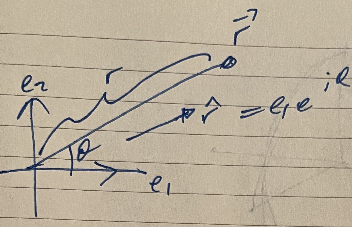
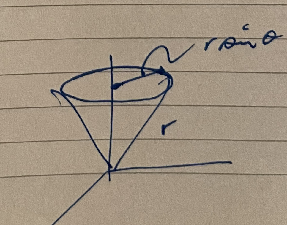
where \( \rcap = \rcap(\phi) \) encodes all the angular dependence of the position vector, and \( r \) is the length along that direction to our point, as illustrated in fig. 1.

fig. 1. Cylindrical coordinates position vector.

The radial unit vector has a compact GA representation
\begin{equation}\label{eqn:amomentum:40}
\rcap = \Be_1 e^{i\phi},
\end{equation}
where \( i = \Be_1 \Be_2 \).

The velocity (or momentum) will have both \( \rcap \) and \( \phicap \) dependence. By chain rule, that velocity is
\begin{equation}\label{eqn:amomentum:60}
\Bv = \dot{r} \rcap + r \dot{\rcap},
\end{equation}
where
\begin{equation}\label{eqn:amomentum:80}
\begin{aligned}
\dot{\rcap}
&= \Be_1 i e^{i\phi} \dot{\phi} \\
&= \Be_2 e^{i\phi} \dot{\phi} \\
&= \phicap \dot{\phi}.
\end{aligned}
\end{equation}
It is left to the reader to show that the vector designated \( \phicap \), is a unit vector and perpendicular to \( \rcap \) (Hint: compute the grade-0 selection of the product of the two to show that they are perpendicular.)

We can now compute the momentum, which is
\begin{equation}\label{eqn:amomentum:100}
\Bp = m \Bv = m \lr{ \dot{r} \rcap + r \dot{\phi} \phicap },
\end{equation}
and the angular momentum bivector
\begin{equation}\label{eqn:amomentum:120}
\begin{aligned}
L
&= \Br \wedge \Bp \\
&= m \lr{ r \rcap } \wedge \lr{ \dot{r} \rcap + r \dot{\phi} \phicap } \\
&= m r^2 \dot{\phi} \rcap \phicap.
\end{aligned}
\end{equation}

This has the \( m r^2 \dot{\phi} \) magnitude that the OP was seeking.

Spherical coordinates.

In spherical coordinates, our position vector is
\begin{equation}\label{eqn:amomentum:140}
\Br = r \lr{ \Be_1 \sin\theta \cos\phi + \Be_2 \sin\theta \sin\phi + \Be_3 \cos\theta },
\end{equation}
as sketched in fig. 2.

fig. 2. Spherical coordinates.

We can factor this into a more compact representation
\begin{equation}\label{eqn:amomentum:160}
\begin{aligned}
\Br
&= r \lr{ \sin\theta \Be_1 (\cos\phi + \Be_{12} \sin\phi ) + \Be_3 \cos\theta } \\
&= r \lr{ \sin\theta \Be_1 e^{\Be_{12} \phi } + \Be_3 \cos\theta } \\
&= r \Be_3 \lr{ \cos\theta + \sin\theta \Be_3 \Be_1 e^{\Be_{12} \phi } }.
\end{aligned}
\end{equation}

It is useful to name two of the bivector terms above, first, we write \( i \) for the azimuthal plane bivector sketched in fig. 3.

Spherical coordinates, azimuthal plane.

\begin{equation}\label{eqn:amomentum:180}
i = \Be_{12},
\end{equation}
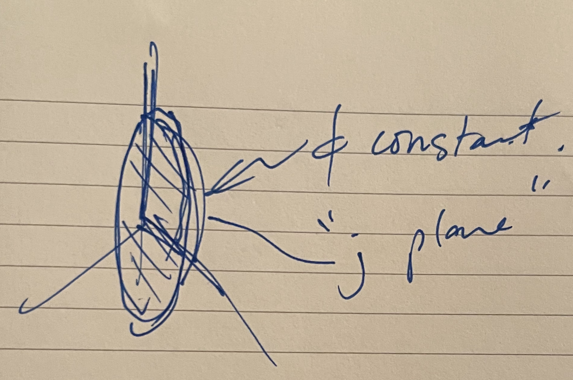
and introduce a bivector \( j \) that encodes the \( \Be_3, \rcap \) plane as sketched in fig. 4.

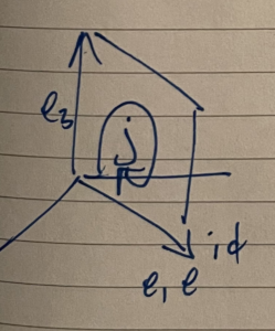
Spherical coordinates, “j-plane”.

\begin{equation}\label{eqn:amomentum:200}
j = \Be_{31} e^{i \phi}.
\end{equation}

Having done so, we now have a compact representation for our position vector
\begin{equation}\label{eqn:amomentum:220}
\begin{aligned}
\Br
&= r \Be_3 \lr{ \cos\theta + j \sin\theta } \\
&= r \Be_3 e^{j \theta}.
\end{aligned}
\end{equation}

This provides us with a nice compact representation of the radial unit vector
\begin{equation}\label{eqn:amomentum:240}
\rcap = \Be_3 e^{j \theta}.
\end{equation}

Just as was the case in cylindrical coordinates, our azimuthal plane unit vector is
\begin{equation}\label{eqn:amomentum:280}
\phicap = \Be_2 e^{i\phi}.
\end{equation}

Now we want to compute the velocity vector. As was the case in cylindrical coordinates, we have
\begin{equation}\label{eqn:amomentum:300}
\Bv = \dot{r} \rcap + r \dot{\rcap},
\end{equation}
but now we need the spherical representation for the \( \rcap \) derivative, which is
\begin{equation}\label{eqn:amomentum:320}
\begin{aligned}
\dot{\rcap}
&=
\PD{\theta}{\rcap} \dot{\theta} + \PD{\phi}{\rcap} \dot{\phi} \\
&=
\Be_3 e^{j\theta} j \dot{\theta} + \Be_3 \sin\theta \PD{\phi}{j} \dot{\phi} \\
&=
\rcap j \dot{\theta} + \Be_3 \sin\theta j i \dot{\phi}.
\end{aligned}
\end{equation}
We can reduce the second multivector term without too much work
\begin{equation}\label{eqn:amomentum:340}
\begin{aligned}
\Be_3 j i
&=
\Be_3 \Be_{31} e^{i\phi} i \\
&=
\Be_3 \Be_{31} i e^{i\phi} \\
&=
\Be_{33112} e^{i\phi} \\
&=
\Be_{2} e^{i\phi} \\
&= \phicap,
\end{aligned}
\end{equation}
so we have
\begin{equation}\label{eqn:amomentum:360}
\dot{\rcap}
=
\rcap j \dot{\theta} + \sin\theta \phicap \dot{\phi}.
\end{equation}

The velocity is
\begin{equation}\label{eqn:amomentum:380}
\Bv = \dot{r} \rcap + r \lr{ \rcap j \dot{\theta} + \sin\theta \phicap \dot{\phi} }.
\end{equation}

Now we can finally compute the angular momentum bivector, which is
\begin{equation}\label{eqn:amomentum:400}
\begin{aligned}
L &=
\Br \wedge \Bp \\
&=
m r \rcap \wedge \lr{ \dot{r} \rcap + r \lr{ \rcap j \dot{\theta} + \sin\theta \phicap \dot{\phi} } } \\
&=
m r^2 \rcap \wedge \lr{ \rcap j \dot{\theta} + \sin\theta \phicap \dot{\phi} } \\
&=
m r^2 \gpgradetwo{ \rcap \lr{ \rcap j \dot{\theta} + \sin\theta \phicap \dot{\phi} } },
\end{aligned}
\end{equation}
which is just
\begin{equation}\label{eqn:amomentum:420}
L =
m r^2 \lr{ j \dot{\theta} + \sin\theta \rcap \phicap \dot{\phi} }.
\end{equation}

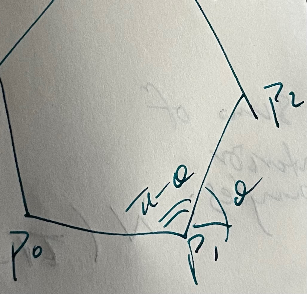
I was slightly surprised by this result, as I naively expected the cylindrical coordinate result. We have a \( m r^2 \rcap \phicap \dot{\phi} \) term, as was the case in cylindrical coordinates, but scaled down with a \( \sin\theta \) factor. However, this result does make sense. Consider for example, some fixed circular motion with \( \theta = \mathrm{constant} \), as sketched in fig. 5.

fig. 5. Circular motion for constant theta

The radius of this circle is actually \( r \sin\theta \), so the total angular momentum for that motion is scaled down to \( m r^2 \sin\theta \dot{\phi} \), smaller than the maximum circular angular momentum of \( m r^2 \dot{\phi} \) which occurs in the \( \theta = \pi/2 \) azimuthal plane. Similarly, if we have circular motion in the “j-plane”, sketched in fig. 6.

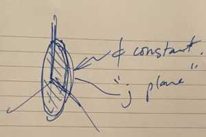
fig. 6. Circular motion for constant phi.

where \( \phi = \mathrm{constant} \), then our angular momentum is \( L = m r^2 j \dot{\theta} \).