[Click here for a PDF of this post with nicer formatting]
Disclaimer
Peeter’s lecture notes from class. These may be incoherent and rough, especially since I didn’t attend this class myself, and am doing a walkthrough of notes provided by Nishant.
These are notes for the UofT course PHY1520, Graduate Quantum Mechanics, taught by Prof. Paramekanti, covering [1] chap. 5 content.
Approximation methods
Suppose we have a perturbed Hamiltonian
\begin{equation}\label{eqn:qmLecture18:20}
H = H_0 + \lambda V,
\end{equation}
where \( \lambda = 0 \) represents a solvable (perhaps known) system, and \( \lambda = 1 \) is the case of interest. There are two approaches of interest
- Direct solution of \( H \) with \( \lambda = 1 \).
- Take \( \lambda \) small, and do a series expansion. This is perturbation theory.
Variational methods
Given
\begin{equation}\label{eqn:qmLecture18:40}
H \ket{\phi_n} = E_n \ket{\phi_n},
\end{equation}
where we don’t know \( \ket{\phi_n} \), we can compute the expectation with respect to an arbitrary state \( \ket{\psi} \)
\begin{equation}\label{eqn:qmLecture18:60}
\bra{\psi} H \ket{\psi}
=
\bra{\psi} H \lr{ \sum_n \ket{\phi_n} \bra{\phi_n} } \ket{\psi}
=
\sum_n E_n \braket{\psi}{\phi_n} \braket{\phi_n}{\psi}
=
\sum_n E_n \Abs{\braket{\psi}{\phi_n}}^2.
\end{equation}
Define
\begin{equation}\label{eqn:qmLecture18:80}
\overline{{E}}
= \frac{\bra{\psi} H \ket{\psi}}{\braket{\psi}{\psi}}.
\end{equation}
Assuming that it is possible to express the state in the Hamiltonian energy basis
\begin{equation}\label{eqn:qmLecture18:100}
\ket{\psi}
=
\sum_n a_n \ket{\phi_n},
\end{equation}
this average energy is
\begin{equation}\label{eqn:qmLecture18:120}
\overline{{E}}
= \frac{ \sum_{m,n}\bra{\phi_m} a_m^\conj H a_n \ket{\phi_n}}{ \sum_n \Abs{a_n}^2 }
= \frac{ \sum_{n} \Abs{a_n}^2 E_n }{ \sum_n \Abs{a_n}^2 }.
= \sum_{n}
\frac{\Abs{a_n}^2 }{ \sum_n \Abs{a_n}^2 }
E_n
= \sum_n \frac{P_n}{\sum_m P_m} E_n,
\end{equation}
where \( P_m = \Abs{a_m}^2 \), which has the structure of a probability coefficient once divided by \( \sum_m P_m \), as sketched in fig. 1.
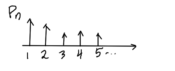
fig. 1. A decreasing probability distribution
This average energy is a probability weighted average of the individual energy basis states. One of those energies is the ground state energy \( E_1 \), so we necessarily have
\begin{equation}\label{eqn:qmLecture18:140}
\boxed{
\overline{{E}} \ge E_1.
}
\end{equation}
Example: particle in a \( [0,L] \) box.
For the infinite potential box sketched in fig. 2.
![fig. 2. Infinite potential [0,L] box.](https://peeterjoot.com/wp-content/uploads/2015/11/lecture18Fig2.png)
fig. 2. Infinite potential [0,L] box.
The exact solutions for such a system are found to be
\begin{equation}\label{eqn:qmLecture18:220}
\psi(x) = \sqrt{\frac{2}{L}} \sin\lr{ \frac{n \pi}{L} x },
\end{equation}
where the energies are
\begin{equation}\label{eqn:qmLecture18:240}
E = \frac{\Hbar^2}{2m} \frac{n^2 \pi^2}{L^2}.
\end{equation}
The function \( \psi’ = x (L-x) \) also satisfies the boundary value constraints? How close in energy is that function to the ground state?
\begin{equation}\label{eqn:qmLecture18:260}
\overline{{E}}
=
-\frac{\Hbar^2}{2m} \frac{\int_0^L dx x (L-x) \frac{d^2}{dx^2} \lr{ x (L-x) }}{
\int_0^L dx x^2 (L-x)^2
}
=
\frac{\Hbar^2}{2m} \frac{\frac{2 L^3}{6}}{
\frac{L^5}{30}
}
=
\frac{\Hbar^2}{2m} \frac{10}{L^2}.
\end{equation}
This average energy is quite close to the ground state energy
\begin{equation}\label{eqn:qmLecture18:280}
\frac{\overline{{E}} }{E_1} = \frac{10}{\pi^2} = 1.014.
\end{equation}
Example II: particle in a \( [-L/2,L/2] \) box.
![fig. 3. Infinite potential [-L/2,L/2] box.](https://peeterjoot.com/wp-content/uploads/2015/11/lecture18Fig3.png)
fig. 3. Infinite potential [-L/2,L/2] box.
Shifting the boundaries, as sketched in fig. 3 doesn’t change the energy levels. For this potential let’s try a shifted trial function
\begin{equation}\label{eqn:qmLecture18:300}
\psi(x) = \lr{ x – \frac{L}{2} } \lr{ x + \frac{L}{2} } = x^2 – \frac{L^2}{4},
\end{equation}
without worrying about the form of the exact solution. This produces the same result as above
\begin{equation}\label{eqn:qmLecture18:270}
\overline{{E}}
=
-\frac{\Hbar^2}{2m} \frac{\int_0^L dx \lr{ x^2 – \frac{L^2}{4} } \frac{d^2}{dx^2} \lr{ x^2 – \frac{L^2}{4} }}{
\int_0^L dx \lr{x^2 – \frac{L^2}{4} }^2
}
=
-\frac{\Hbar^2}{2m} \frac{- 2 L^3/6}{
\frac{L^5}{30}
}
=
\frac{\Hbar^2}{2m} \frac{10}{L^2}.
\end{equation}
Summary (Nishant)
The above example is that of a particle in a box. The actual wave function is a sin as shown. But we can
come up with a guess wave function that meets the boundary conditions and ask how accurate it is
compared to the actual one.
Basically we are assuming a wave function form and then seeing how it differs from the exact form.
We cannot do this if we have nothing to compare it against. But, we note that the variance of the
number operator in the systems eigenstate is zero. So we can still calculate the variance and try to
minimize it. This is one way of coming up with an approximate wave function. This does not necessarily
give the ground state wave function though. For this we need to minimize the energy itself.
References
[1] Jun John Sakurai and Jim J Napolitano. Modern quantum mechanics. Pearson Higher Ed, 2014.