[If mathjax doesn’t display properly for you, click here for a PDF of this post]
This post logically follows both of the following:
- Curvilinear coordinates and gradient in spacetime, and reciprocal frames, and
- Lorentz transformations in Space Time Algebra (STA)
The PDF linked above above contains all the content from this post plus (1.) above [to be edited later into a more logical sequence.]
More examples.
Here are a few additional examples of reciprocal frame calculations.
Problem: Unidirectional arbitrary functional dependence.
Let
\begin{equation}\label{eqn:reciprocal:2540}
x = a f(u),
\end{equation}
where \( a \) is a constant vector and \( f(u)\) is some arbitrary differentiable function with a non-zero derivative in the region of interest.
Answer
Here we have just a single tangent space direction (a line in spacetime) with tangent vector
\begin{equation}\label{eqn:reciprocal:2400}
\Bx_u = a \PD{u}{f} = a f_u,
\end{equation}
so we see that the tangent space vectors are just rescaled values of the direction vector \( a \).
This is a simple enough parameterization that we can compute the reciprocal frame vector explicitly using the gradient. We expect that \( \Bx^u = 1/\Bx_u \), and find
\begin{equation}\label{eqn:reciprocal:2420}
\inv{a} \cdot x = f(u),
\end{equation}
but for constant \( a \), we know that \( \grad a \cdot x = a \), so taking gradients of both sides we find
\begin{equation}\label{eqn:reciprocal:2440}
\inv{a} = \grad f = \PD{u}{f} \grad u,
\end{equation}
so the reciprocal vector is
\begin{equation}\label{eqn:reciprocal:2460}
\Bx^u = \grad u = \inv{a f_u},
\end{equation}
as expected.
Problem: Linear two variable parameterization.
Let \( x = a u + b v \), where \( x \wedge a \wedge b = 0 \) represents spacetime plane (also the tangent space.) Find the curvilinear coordinates and their reciprocals.
Answer
The frame vectors are easy to compute, as they are just
\begin{equation}\label{eqn:reciprocal:1960}
\begin{aligned}
\Bx_u &= \PD{u}{x} = a \\
\Bx_v &= \PD{v}{x} = b.
\end{aligned}
\end{equation}
This is an example of a parametric equation that we can easily invert, as we have
\begin{equation}\label{eqn:reciprocal:1980}
\begin{aligned}
x \wedge a &= – v \lr{ a \wedge b } \\
x \wedge b &= u \lr{ a \wedge b },
\end{aligned}
\end{equation}
so
\begin{equation}\label{eqn:reciprocal:2000}
\begin{aligned}
u
&= \inv{ a \wedge b } \cdot \lr{ x \wedge b } \\
&= \inv{ \lr{a \wedge b}^2 } \lr{ a \wedge b } \cdot \lr{ x \wedge b } \\
&=
\frac{
\lr{b \cdot x} \lr{ a \cdot b }
–
\lr{a \cdot x} \lr{ b \cdot b }
}{ \lr{a \wedge b}^2 }
\end{aligned}
\end{equation}
\begin{equation}\label{eqn:reciprocal:2020}
\begin{aligned}
v &= -\inv{ a \wedge b } \cdot \lr{ x \wedge a } \\
&= -\inv{ \lr{a \wedge b}^2 } \lr{ a \wedge b } \cdot \lr{ x \wedge a } \\
&=
-\frac{
\lr{b \cdot x} \lr{ a \cdot a }
–
\lr{a \cdot x} \lr{ a \cdot b }
}{ \lr{a \wedge b}^2 }
\end{aligned}
\end{equation}
Recall that \( \grad \lr{ a \cdot x} = a \), if \( a \) is a constant, so our gradients are just
\begin{equation}\label{eqn:reciprocal:2040}
\begin{aligned}
\grad u
&=
\frac{
b \lr{ a \cdot b }
–
a
\lr{ b \cdot b }
}{ \lr{a \wedge b}^2 } \\
&=
b \cdot \inv{ a \wedge b },
\end{aligned}
\end{equation}
and
\begin{equation}\label{eqn:reciprocal:2060}
\begin{aligned}
\grad v
&=
-\frac{
b \lr{ a \cdot a }
–
a \lr{ a \cdot b }
}{ \lr{a \wedge b}^2 } \\
&=
-a \cdot \inv{ a \wedge b }.
\end{aligned}
\end{equation}
Expressed in terms of the frame vectors, this is just
\begin{equation}\label{eqn:reciprocal:2080}
\begin{aligned}
\Bx^u &= \Bx_v \cdot \inv{ \Bx_u \wedge \Bx_v } \\
\Bx^v &= -\Bx_u \cdot \inv{ \Bx_u \wedge \Bx_v },
\end{aligned}
\end{equation}
so we were able to show, for this special two parameter linear case, that the explicit evaluation of the gradients has the exact structure that we intuited that the reciprocals must have, provided they are constrained to the spacetime plane \( a \wedge b \). It is interesting to observe how this structure falls out of the linear system solution so directly. Also note that these reciprocals are not defined at the origin of the \( (u,v) \) parameter space.
Problem: Quadratic two variable parameterization.
Now consider a variation of the previous problem, with \( x = a u^2 + b v^2 \). Find the curvilinear coordinates and their reciprocals.
Answer
\begin{equation}\label{eqn:reciprocal:2100}
\begin{aligned}
\Bx_u &= \PD{u}{x} = 2 u a \\
\Bx_v &= \PD{v}{x} = 2 v b.
\end{aligned}
\end{equation}
Our tangent space is still the \( a \wedge b \) plane (as is the surface itself), but the spacing of the cells starts getting wider in proportion to \( u, v \).
Utilizing the work from the previous problem, we have
\begin{equation}\label{eqn:reciprocal:2120}
\begin{aligned}
2 u \grad u &=
b \cdot \inv{ a \wedge b } \\
2 v \grad v &=
-a \cdot \inv{ a \wedge b }.
\end{aligned}
\end{equation}
A bit of rearrangement can show that this is equivalent to the reciprocal frame identities. This is a second demonstration that the gradient and the algebraic formulations for the reciprocals match, at least for these special cases of linear non-coupled parameterizations.
Problem: Reciprocal frame for generalized cylindrical parameterization.
Let the vector parameterization be \( x(\rho,\theta) = \rho e^{-i\theta/2} x(\rho_0, \theta_0) e^{i \theta} \), where \( i^2 = \pm 1 \) is a unit bivector (\(+1\) for a boost, and \(-1\) for a rotation), and where \(\theta, \rho\) are scalars. Find the tangent space vectors and their reciprocals.
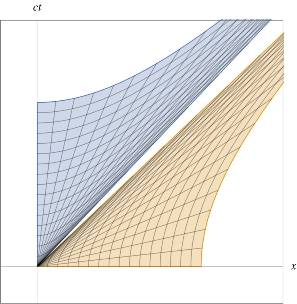
Note that this is cylindrical parameterization for the rotation case, and traces out hyperbolic regions for the boost case. The boost case is illustrated in fig. 1 where hyperbolas in the light cone are found for boosts of \( \gamma_0\) with various values of \(\rho\), and the spacelike hyperbolas are boosts of \( \gamma_1 \), again for various values of \( \rho \).
Answer
The tangent space vectors are
\begin{equation}\label{eqn:reciprocal:2480}
\Bx_\rho = \frac{x}{\rho},
\end{equation}
and
\begin{equation}\label{eqn:reciprocal:2500}
\begin{aligned}
\Bx_\theta
&= -\frac{i}{2} x + x \frac{i}{2} \\
&= x \cdot i.
\end{aligned}
\end{equation}
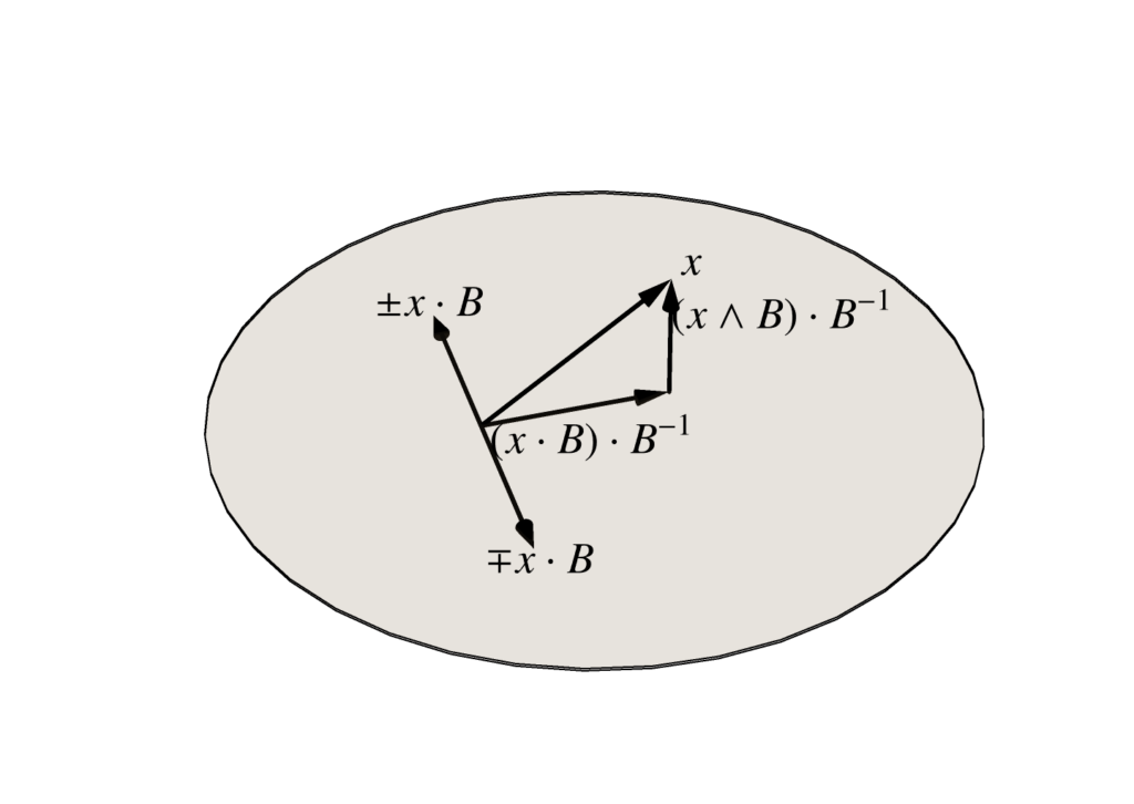
Recall that \( x \cdot i \) lies perpendicular to \( x \) (in the plane \( i \)), as illustrated in fig. 2. This means that \( \Bx_\rho \) and \( \Bx_\theta \) are orthogonal, so we can find the reciprocal vectors by just inverting them
\begin{equation}\label{eqn:reciprocal:2520}
\begin{aligned}
\Bx^\rho &= \frac{\rho}{x} \\
\Bx^\theta &= \frac{1}{x \cdot i}.
\end{aligned}
\end{equation}
Parameterization of a general linear transformation.
Given \( N \) parameters \( u^0, u^1, \cdots u^{N-1} \), a general linear transformation from the parameter space to the vector space has the form
\begin{equation}\label{eqn:reciprocal:2160}
x =
{a^\alpha}_\beta \gamma_\alpha u^\beta,
\end{equation}
where \( \beta \in [0, \cdots, N-1] \) and \( \alpha \in [0,3] \).
For such a general transformation, observe that the curvilinear basis vectors are
\begin{equation}\label{eqn:reciprocal:2180}
\begin{aligned}
\Bx_\mu
&= \PD{u^\mu}{x} \\
&= \PD{u^\mu}{}
{a^\alpha}_\beta \gamma_\alpha u^\beta \\
&=
{a^\alpha}_\mu \gamma_\alpha.
\end{aligned}
\end{equation}
We find an interpretation of \( {a^\alpha}_\mu \) by dotting \( \Bx_\mu \) with the reciprocal frame vectors of the standard basis
\begin{equation}\label{eqn:reciprocal:2200}
\begin{aligned}
\Bx_\mu \cdot \gamma^\nu
&=
{a^\alpha}_\mu \lr{ \gamma_\alpha \cdot \gamma^\nu } \\
&=
{a^\nu}_\mu,
\end{aligned}
\end{equation}
so
\begin{equation}\label{eqn:reciprocal:2220}
x = \Bx_\mu u^\mu.
\end{equation}
We are able to reinterpret \ref{eqn:reciprocal:2160} as a contraction of the tangent space vectors with the parameters, scaling and summing these direction vectors to characterize all the points in the tangent plane.
Theorem 1.1: Projecting onto the tangent space.
\begin{equation}\label{eqn:reciprocal:2560}
\textrm{Proj}_{\textrm{T}} y = \lr{ y \cdot \Bx^\mu } \Bx_\mu = \lr{ y \cdot \Bx_\mu } \Bx^\mu.
\end{equation}
Start proof:
Let’s designate \( a \) as the portion of the vector \( y \) that lies outside of the tangent space
\begin{equation}\label{eqn:reciprocal:2260}
y = y^\mu \Bx_\mu + a.
\end{equation}
If we knew the coordinates \( y^\mu \), we would have a recipe for the projection.
Algebraically, requiring that \( a \) lies outside of the tangent space, is equivalent to stating \( a \cdot \Bx_\mu = a \cdot \Bx^\mu = 0 \). We use that fact, and then take dot products
\begin{equation}\label{eqn:reciprocal:2280}
\begin{aligned}
y \cdot \Bx^\nu
&= \lr{ y^\mu \Bx_\mu + a } \cdot \Bx^\nu \\
&= y^\nu,
\end{aligned}
\end{equation}
so
\begin{equation}\label{eqn:reciprocal:2300}
y = \lr{ y \cdot \Bx^\mu } \Bx_\mu + a.
\end{equation}
Similarly, the tangent space projection can be expressed as a linear combination of reciprocal basis elements
\begin{equation}\label{eqn:reciprocal:2320}
y = y_\mu \Bx^\mu + a.
\end{equation}
Dotting with \( \Bx_\mu \), we have
\begin{equation}\label{eqn:reciprocal:2340}
\begin{aligned}
y \cdot \Bx^\mu
&= \lr{ y_\alpha \Bx^\alpha + a } \cdot \Bx_\mu \\
&= y_\mu,
\end{aligned}
\end{equation}
so
\begin{equation}\label{eqn:reciprocal:2360}
y = \lr{ y \cdot \Bx^\mu } \Bx_\mu + a.
\end{equation}
We find the two stated ways of computing the projection.
Observe that, for the special case that all of \( \setlr{ \Bx_\mu } \) are orthogonal, the equivalence of these two projection methods follows directly, since
\begin{equation}\label{eqn:reciprocal:2380}
\begin{aligned}
\lr{ y \cdot \Bx^\mu } \Bx_\mu
&=
\lr{ y \cdot \inv{\Bx_\mu} } \inv{\Bx^\mu} \\
&=
\lr{ y \cdot \frac{\Bx_\mu}{\lr{\Bx_\mu}^2 } } \frac{\Bx^\mu}{\lr{\Bx^\mu}^2} \\
&=
\lr{ y \cdot \Bx_\mu } \Bx^\mu.
\end{aligned}
\end{equation}


