[Click here for a PDF of this post with nicer formatting]
Stokes Theorem
The Fundamental Theorem of (Geometric) Calculus is a generalization of Stokes theorem to multivector integrals. Notationally, it looks like Stokes theorem with all the dot and wedge products removed. It is worth restating Stokes theorem and all the definitions associated with it for reference
Stokes’ Theorem
For blades \(F \in \bigwedge^{s}\), and \(m\) volume element \(d^k \Bx, s < k\), \begin{equation*} \int_V d^k \Bx \cdot (\boldpartial \wedge F) = \oint_{\partial V} d^{k-1} \Bx \cdot F. \end{equation*} This is a loaded and abstract statement, and requires many definitions to make it useful
- The volume integral is over a \(m\) dimensional surface (manifold).
- Integration over the boundary of the manifold \(V\) is indicated by \( \partial V \).
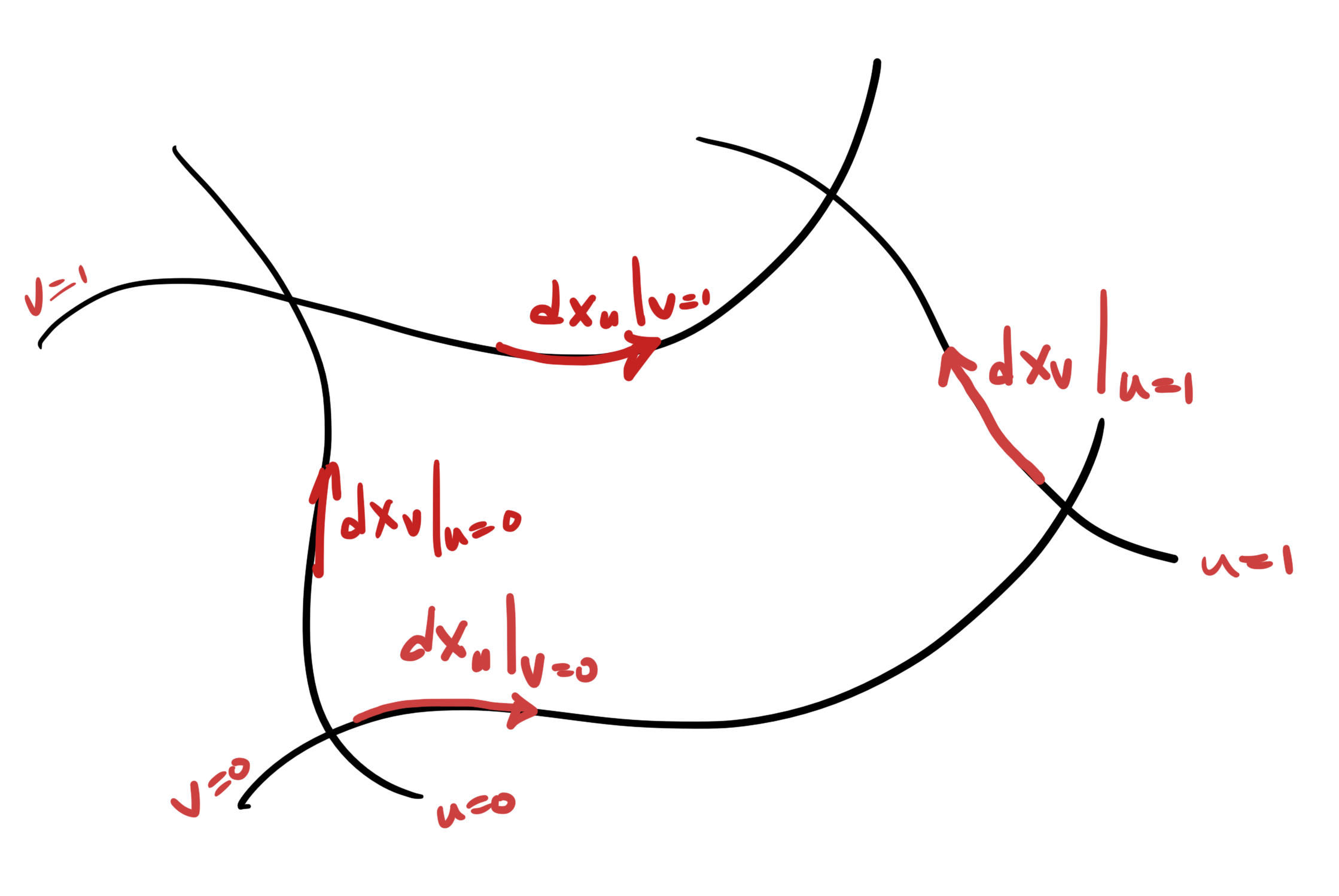
- This manifold is assumed to be spanned by a parameterized vector \( \Bx(u^1, u^2, \cdots, u^k) \).
- A curvilinear coordinate basis \( \setlr{ \Bx_i } \) can be defined on the manifold by
\begin{equation}\label{eqn:fundamentalTheoremOfCalculus:40}
\Bx_i \equiv \PD{u^i}{\Bx} \equiv \partial_i \Bx.
\end{equation} - A dual basis \( \setlr{\Bx^i} \) reciprocal to the tangent vector basis \( \Bx_i \) can be calculated subject to the requirement \( \Bx_i \cdot \Bx^j = \delta_i^j \).
- The vector derivative \(\boldpartial\), the projection of the gradient onto the tangent space of the manifold, is defined by
\begin{equation}\label{eqn:fundamentalTheoremOfCalculus:100}
\boldpartial = \Bx^i \partial_i = \sum_{i=1}^k \Bx_i \PD{u^i}{}.
\end{equation} - The volume element is defined by
\begin{equation}\label{eqn:fundamentalTheoremOfCalculus:60}
d^k \Bx = d\Bx_1 \wedge d\Bx_2 \cdots \wedge d\Bx_k,
\end{equation}where
\begin{equation}\label{eqn:fundamentalTheoremOfCalculus:80}
d\Bx_k = \Bx_k du^k,\qquad \text{(no sum)}.
\end{equation} - The volume element is non-zero on the manifold, or \( \Bx_1 \wedge \cdots \wedge \Bx_k \ne 0 \).
- The surface area element \( d^{k-1} \Bx \), is defined by
\begin{equation}\label{eqn:fundamentalTheoremOfCalculus:120}
d^{k-1} \Bx = \sum_{i = 1}^k (-1)^{k-i} d\Bx_1 \wedge d\Bx_2 \cdots \widehat{d\Bx_i} \cdots \wedge d\Bx_k,
\end{equation}where \( \widehat{d\Bx_i} \) indicates the omission of \( d\Bx_i \).
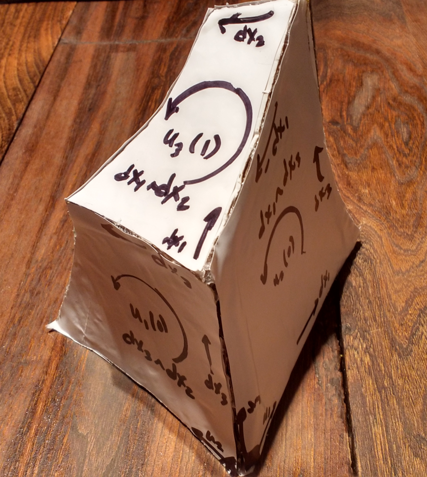
- My proof for this theorem was restricted to a simple “rectangular” volume parameterized by the ranges
\(
[u^1(0), u^1(1) ] \otimes
[u^2(0), u^2(1) ] \otimes \cdots \otimes
[u^k(0), u^k(1) ] \) - The precise meaning that should be given to oriented area integral is
\begin{equation}\label{eqn:fundamentalTheoremOfCalculus:140}
\oint_{\partial V} d^{k-1} \Bx \cdot F
=
\sum_{i = 1}^k (-1)^{k-i} \int \evalrange{
\lr{ \lr{ d\Bx_1 \wedge d\Bx_2 \cdots \widehat{d\Bx_i} \cdots \wedge d\Bx_k } \cdot F }
}{u^i = u^i(0)}{u^i(1)},
\end{equation}where both the a area form and the blade \( F \) are evaluated at the end points of the parameterization range.
After the work of stating exactly what is meant by this theorem, most of the proof follows from the fact that for \( s < k \) the volume curl dot product can be expanded as \begin{equation}\label{eqn:fundamentalTheoremOfCalculus:160} \int_V d^k \Bx \cdot (\boldpartial \wedge F) = \int_V d^k \Bx \cdot (\Bx^i \wedge \partial_i F) = \int_V \lr{ d^k \Bx \cdot \Bx^i } \cdot \partial_i F. \end{equation} Each of the \(du^i\) integrals can be evaluated directly, since each of the remaining \(d\Bx_j = du^j \PDi{u^j}{}, i \ne j \) is calculated with \( u^i \) held fixed. This allows for the integration over a ``rectangular'' parameterization region, proving the theorem for such a volume parameterization. A more general proof requires a triangulation of the volume and surface, but the basic principle of the theorem is evident, without that additional work.
Fundamental Theorem of Calculus
There is a Geometric Algebra generalization of Stokes theorem that does not have the blade grade restriction of Stokes theorem. In [2] this is stated as
\begin{equation}\label{eqn:fundamentalTheoremOfCalculus:180}
\int_V d^k \Bx \boldpartial F = \oint_{\partial V} d^{k-1} \Bx F.
\end{equation}
A similar expression is used in [1] where it is also pointed out there is a variant with the vector derivative acting to the left
\begin{equation}\label{eqn:fundamentalTheoremOfCalculus:200}
\int_V F d^k \Bx \boldpartial = \oint_{\partial V} F d^{k-1} \Bx.
\end{equation}
In [3] it is pointed out that a bidirectional formulation is possible, providing the most general expression of the Fundamental Theorem of (Geometric) Calculus
\begin{equation}\label{eqn:fundamentalTheoremOfCalculus:220}
\boxed{
\int_V F d^k \Bx \boldpartial G = \oint_{\partial V} F d^{k-1} \Bx G.
}
\end{equation}
Here the vector derivative acts both to the left and right on \( F \) and \( G \). The specific action of this operator is
\begin{equation}\label{eqn:fundamentalTheoremOfCalculus:240}
\begin{aligned}
F \boldpartial G
&=
(F \boldpartial) G
+
F (\boldpartial G) \\
&=
(\partial_i F) \Bx^i G
+
F \Bx^i (\partial_i G).
\end{aligned}
\end{equation}
The fundamental theorem can be demonstrated by direct expansion. With the vector derivative \( \boldpartial \) and its partials \( \partial_i \) acting bidirectionally, that is
\begin{equation}\label{eqn:fundamentalTheoremOfCalculus:260}
\begin{aligned}
\int_V F d^k \Bx \boldpartial G
&=
\int_V F d^k \Bx \Bx^i \partial_i G \\
&=
\int_V F \lr{ d^k \Bx \cdot \Bx^i + d^k \Bx \wedge \Bx^i } \partial_i G.
\end{aligned}
\end{equation}
Both the reciprocal frame vectors and the curvilinear basis span the tangent space of the manifold, since we can write any reciprocal frame vector as a set of projections in the curvilinear basis
\begin{equation}\label{eqn:fundamentalTheoremOfCalculus:280}
\Bx^i = \sum_j \lr{ \Bx^i \cdot \Bx^j } \Bx_j,
\end{equation}
so \( \Bx^i \in sectionpan \setlr{ \Bx_j, j \in [1,k] } \).
This means that \( d^k \Bx \wedge \Bx^i = 0 \), and
\begin{equation}\label{eqn:fundamentalTheoremOfCalculus:300}
\begin{aligned}
\int_V F d^k \Bx \boldpartial G
&=
\int_V F \lr{ d^k \Bx \cdot \Bx^i } \partial_i G \\
&=
\sum_{i = 1}^{k}
\int_V
du^1 du^2 \cdots \widehat{ du^i} \cdots du^k
F \lr{
(-1)^{k-i}
\Bx_1 \wedge \Bx_2 \cdots \widehat{\Bx_i} \cdots \wedge \Bx_k } \partial_i G du^i \\
&=
\sum_{i = 1}^{k}
(-1)^{k-i}
\int_{u^1}
\int_{u^2}
\cdots
\int_{u^{i-1}}
\int_{u^{i+1}}
\cdots
\int_{u^k}
\evalrange{ \lr{
F d\Bx_1 \wedge d\Bx_2 \cdots \widehat{d\Bx_i} \cdots \wedge d\Bx_k G
}
}{u^i = u^i(0)}{u^i(1)}.
\end{aligned}
\end{equation}
Adding in the same notational sugar that we used in Stokes theorem, this proves the Fundamental theorem \ref{eqn:fundamentalTheoremOfCalculus:220} for “rectangular” parameterizations. Note that such a parameterization need not actually be rectangular.
Example: Application to Maxwell’s equation
{example:fundamentalTheoremOfCalculus:1}
Maxwell’s equation is an example of a first order gradient equation
\begin{equation}\label{eqn:fundamentalTheoremOfCalculus:320}
\grad F = \inv{\epsilon_0 c} J.
\end{equation}
Integrating over a four-volume (where the vector derivative equals the gradient), and applying the Fundamental theorem, we have
\begin{equation}\label{eqn:fundamentalTheoremOfCalculus:340}
\inv{\epsilon_0 c} \int d^4 x J = \oint d^3 x F.
\end{equation}
Observe that the surface area element product with \( F \) has both vector and trivector terms. This can be demonstrated by considering some examples
\begin{equation}\label{eqn:fundamentalTheoremOfCalculus:360}
\begin{aligned}
\gamma_{012} \gamma_{01} &\propto \gamma_2 \\
\gamma_{012} \gamma_{23} &\propto \gamma_{023}.
\end{aligned}
\end{equation}
On the other hand, the four volume integral of \( J \) has only trivector parts. This means that the integral can be split into a pair of same-grade equations
\begin{equation}\label{eqn:fundamentalTheoremOfCalculus:380}
\begin{aligned}
\inv{\epsilon_0 c} \int d^4 x \cdot J &=
\oint \gpgradethree{ d^3 x F} \\
0 &=
\oint d^3 x \cdot F.
\end{aligned}
\end{equation}
The first can be put into a slightly tidier form using a duality transformation
\begin{equation}\label{eqn:fundamentalTheoremOfCalculus:400}
\begin{aligned}
\gpgradethree{ d^3 x F}
&=
-\gpgradethree{ d^3 x I^2 F} \\
&=
\gpgradethree{ I d^3 x I F} \\
&=
(I d^3 x) \wedge (I F).
\end{aligned}
\end{equation}
Letting \( n \Abs{d^3 x} = I d^3 x \), this gives
\begin{equation}\label{eqn:fundamentalTheoremOfCalculus:420}
\oint \Abs{d^3 x} n \wedge (I F) = \inv{\epsilon_0 c} \int d^4 x \cdot J.
\end{equation}
Note that this normal is normal to a three-volume subspace of the spacetime volume. For example, if one component of that spacetime surface area element is \( \gamma_{012} c dt dx dy \), then the normal to that area component is \( \gamma_3 \).
A second set of duality transformations
\begin{equation}\label{eqn:fundamentalTheoremOfCalculus:440}
\begin{aligned}
n \wedge (IF)
&=
\gpgradethree{ n I F} \\
&=
-\gpgradethree{ I n F} \\
&=
-\gpgradethree{ I (n \cdot F)} \\
&=
-I (n \cdot F),
\end{aligned}
\end{equation}
and
\begin{equation}\label{eqn:fundamentalTheoremOfCalculus:460}
\begin{aligned}
I d^4 x \cdot J
&=
\gpgradeone{ I d^4 x \cdot J } \\
&=
\gpgradeone{ I d^4 x J } \\
&=
\gpgradeone{ (I d^4 x) J } \\
&=
(I d^4 x) J,
\end{aligned}
\end{equation}
can further tidy things up, leaving us with
\begin{equation}\label{eqn:fundamentalTheoremOfCalculus:500}
\boxed{
\begin{aligned}
\oint \Abs{d^3 x} n \cdot F &= \inv{\epsilon_0 c} \int (I d^4 x) J \\
\oint d^3 x \cdot F &= 0.
\end{aligned}
}
\end{equation}
The Fundamental theorem of calculus immediately provides relations between the Faraday bivector \( F \) and the four-current \( J \).
References
[1] C. Doran and A.N. Lasenby. Geometric algebra for physicists. Cambridge University Press New York, Cambridge, UK, 1st edition, 2003.
[2] A. Macdonald. Vector and Geometric Calculus. CreateSpace Independent Publishing Platform, 2012.
[3] Garret Sobczyk and Omar Le\’on S\’anchez. Fundamental theorem of calculus. Advances in Applied Clifford Algebras, 21\penalty0 (1):\penalty0 221–231, 2011. URL https://arxiv.org/abs/0809.4526.