Fundamental Theorem of Geometric Calculus

A multivector Lagrangian for Maxwell’s equation: A summary of previous exploration.

June 21, 2022 math and physics play , , , , , , , , , , , , , , , , , , , ,

This summarizes the significant parts of the last 8 blog posts.

[Click here for a PDF version of this post]

STA form of Maxwell’s equation.

Maxwell’s equations, with electric and fictional magnetic sources (useful for antenna theory and other engineering applications), are
\begin{equation}\label{eqn:maxwellLagrangian:220}
\begin{aligned}
\spacegrad \cdot \BE &= \frac{\rho}{\epsilon} \\
\spacegrad \cross \BE &= – \BM – \mu \PD{t}{\BH} \\
\spacegrad \cdot \BH &= \frac{\rho_\txtm}{\mu} \\
\spacegrad \cross \BH &= \BJ + \epsilon \PD{t}{\BE}.
\end{aligned}
\end{equation}
We can assemble these into a single geometric algebra equation,
\begin{equation}\label{eqn:maxwellLagrangian:240}
\lr{ \spacegrad + \inv{c} \PD{t}{} } F = \eta \lr{ c \rho – \BJ } + I \lr{ c \rho_{\mathrm{m}} – \BM },
\end{equation}
where \( F = \BE + \eta I \BH = \BE + I c \BB \), \( c = 1/\sqrt{\mu\epsilon}, \eta = \sqrt{(\mu/\epsilon)} \).

By multiplying through by \( \gamma_0 \), making the identification \( \Be_k = \gamma_k \gamma_0 \), and
\begin{equation}\label{eqn:maxwellLagrangian:300}
\begin{aligned}
J^0 &= \frac{\rho}{\epsilon}, \quad J^k = \eta \lr{ \BJ \cdot \Be_k }, \quad J = J^\mu \gamma_\mu \\
M^0 &= c \rho_{\mathrm{m}}, \quad M^k = \BM \cdot \Be_k, \quad M = M^\mu \gamma_\mu \\
\grad &= \gamma^\mu \partial_\mu,
\end{aligned}
\end{equation}
we find the STA form of Maxwell’s equation, including magnetic sources
\begin{equation}\label{eqn:maxwellLagrangian:320}
\grad F = J – I M.
\end{equation}

Decoupling the electric and magnetic fields and sources.

We can utilize two separate four-vector potential fields to split Maxwell’s equation into two parts. Let
\begin{equation}\label{eqn:maxwellLagrangian:1740}
F = F_{\mathrm{e}} + I F_{\mathrm{m}},
\end{equation}
where
\begin{equation}\label{eqn:maxwellLagrangian:1760}
\begin{aligned}
F_{\mathrm{e}} &= \grad \wedge A \\
F_{\mathrm{m}} &= \grad \wedge K,
\end{aligned}
\end{equation}
and \( A, K \) are independent four-vector potential fields. Plugging this into Maxwell’s equation, and employing a duality transformation, gives us two coupled vector grade equations
\begin{equation}\label{eqn:maxwellLagrangian:1780}
\begin{aligned}
\grad \cdot F_{\mathrm{e}} – I \lr{ \grad \wedge F_{\mathrm{m}} } &= J \\
\grad \cdot F_{\mathrm{m}} + I \lr{ \grad \wedge F_{\mathrm{e}} } &= M.
\end{aligned}
\end{equation}
However, since \( \grad \wedge F_{\mathrm{m}} = \grad \wedge F_{\mathrm{e}} = 0 \), by construction, the curls above are killed. We may also add in \( \grad \wedge F_{\mathrm{e}} = 0 \) and \( \grad \wedge F_{\mathrm{m}} = 0 \) respectively, yielding two independent gradient equations
\begin{equation}\label{eqn:maxwellLagrangian:1810}
\begin{aligned}
\grad F_{\mathrm{e}} &= J \\
\grad F_{\mathrm{m}} &= M,
\end{aligned}
\end{equation}
one for each of the electric and magnetic sources and their associated fields.

Tensor formulation.

The electromagnetic field \( F \), is a vector-bivector multivector in the multivector representation of Maxwell’s equation, but is a bivector in the STA representation. The split of \( F \) into it’s electric and magnetic field components is observer dependent, but we may write it without reference to a specific observer frame as
\begin{equation}\label{eqn:maxwellLagrangian:1830}
F = \inv{2} \gamma_\mu \wedge \gamma_\nu F^{\mu\nu},
\end{equation}
where \( F^{\mu\nu} \) is an arbitrary antisymmetric 2nd rank tensor. Maxwell’s equation has a vector and trivector component, which may be split out explicitly using grade selection, to find
\begin{equation}\label{eqn:maxwellLagrangian:360}
\begin{aligned}
\grad \cdot F &= J \\
\grad \wedge F &= -I M.
\end{aligned}
\end{equation}
Further dotting and wedging these equations with \( \gamma^\mu \) allows for extraction of scalar relations
\begin{equation}\label{eqn:maxwellLagrangian:460}
\partial_\nu F^{\nu\mu} = J^{\mu}, \quad \partial_\nu G^{\nu\mu} = M^{\mu},
\end{equation}
where \( G^{\mu\nu} = -(1/2) \epsilon^{\mu\nu\alpha\beta} F_{\alpha\beta} \) is also an antisymmetric 2nd rank tensor.

If we treat \( F^{\mu\nu} \) and \( G^{\mu\nu} \) as independent fields, this pair of equations is the coordinate equivalent to \ref{eqn:maxwellLagrangian:1760}, also decoupling the electric and magnetic source contributions to Maxwell’s equation.

Coordinate representation of the Lagrangian.

As observed above, we may choose to express the decoupled fields as curls \( F_{\mathrm{e}} = \grad \wedge A \) or \( F_{\mathrm{m}} = \grad \wedge K \). The coordinate expansion of either field component, given such a representation, is straight forward. For example
\begin{equation}\label{eqn:maxwellLagrangian:1850}
\begin{aligned}
F_{\mathrm{e}}
&= \lr{ \gamma_\mu \partial^\mu } \wedge \lr{ \gamma_\nu A^\nu } \\
&= \inv{2} \lr{ \gamma_\mu \wedge \gamma_\nu } \lr{ \partial^\mu A^\nu – \partial^\nu A^\mu }.
\end{aligned}
\end{equation}

We make the identification \( F^{\mu\nu} = \partial^\mu A^\nu – \partial^\nu A^\mu \), the usual definition of \( F^{\mu\nu} \) in the tensor formalism. In that tensor formalism, the Maxwell Lagrangian is
\begin{equation}\label{eqn:maxwellLagrangian:1870}
\LL = – \inv{4} F_{\mu\nu} F^{\mu\nu} – A_\mu J^\mu.
\end{equation}
We may show this though application of the Euler-Lagrange equations
\begin{equation}\label{eqn:maxwellLagrangian:600}
\PD{A_\mu}{\LL} = \partial_\nu \PD{(\partial_\nu A_\mu)}{\LL}.
\end{equation}
\begin{equation}\label{eqn:maxwellLagrangian:1930}
\begin{aligned}
\PD{(\partial_\nu A_\mu)}{\LL}
&= -\inv{4} (2) \lr{ \PD{(\partial_\nu A_\mu)}{F_{\alpha\beta}} } F^{\alpha\beta} \\
&= -\inv{2} \delta^{[\nu\mu]}_{\alpha\beta} F^{\alpha\beta} \\
&= -\inv{2} \lr{ F^{\nu\mu} – F^{\mu\nu} } \\
&= F^{\mu\nu}.
\end{aligned}
\end{equation}
So \( \partial_\nu F^{\nu\mu} = J^\mu \), the equivalent of \( \grad \cdot F = J \), as expected.

Coordinate-free representation and variation of the Lagrangian.

Because
\begin{equation}\label{eqn:maxwellLagrangian:200}
F^2 =
-\inv{2}
F^{\mu\nu} F_{\mu\nu}
+
\lr{ \gamma_\alpha \wedge \gamma^\beta }
F_{\alpha\mu}
F^{\beta\mu}
+
\frac{I}{4}
\epsilon_{\mu\nu\alpha\beta} F^{\mu\nu} F^{\alpha\beta},
\end{equation}
we may express the Lagrangian \ref{eqn:maxwellLagrangian:1870} in a coordinate free representation
\begin{equation}\label{eqn:maxwellLagrangian:1890}
\LL = \inv{2} F \cdot F – A \cdot J,
\end{equation}
where \( F = \grad \wedge A \).

We will now show that it is also possible to apply the variational principle to the following multivector Lagrangian
\begin{equation}\label{eqn:maxwellLagrangian:1910}
\LL = \inv{2} F^2 – A \cdot J,
\end{equation}
and recover the geometric algebra form \( \grad F = J \) of Maxwell’s equation in it’s entirety, including both vector and trivector components in one shot.

We will need a few geometric algebra tools to do this.

The first such tool is the notational freedom to let the gradient act bidirectionally on multivectors to the left and right. We will designate such action with over-arrows, sometimes also using braces to limit the scope of the action in question. If \( Q, R \) are multivectors, then the bidirectional action of the gradient in a \( Q, R \) sandwich is
\begin{equation}\label{eqn:maxwellLagrangian:1950}
\begin{aligned}
Q \lrgrad R
&= Q \lgrad R + Q \rgrad R \\
&= \lr{ Q \gamma^\mu \lpartial_\mu } R + Q \lr{ \gamma^\mu \rpartial_\mu R } \\
&= \lr{ \partial_\mu Q } \gamma^\mu R + Q \gamma^\mu \lr{ \partial_\mu R }.
\end{aligned}
\end{equation}
In the final statement, the partials are acting exclusively on \( Q \) and \( R \) respectively, but the \( \gamma^\mu \) factors must remain in place, as they do not necessarily commute with any of the multivector factors.

This bidirectional action is a critical aspect of the Fundamental Theorem of Geometric calculus, another tool that we will require. The specific form of that theorem that we will utilize here is
\begin{equation}\label{eqn:maxwellLagrangian:1970}
\int_V Q d^4 \Bx \lrgrad R = \int_{\partial V} Q d^3 \Bx R,
\end{equation}
where \( d^4 \Bx = I d^4 x \) is the pseudoscalar four-volume element associated with a parameterization of space time. For our purposes, we may assume that parameterization are standard basis coordinates associated with the basis \( \setlr{ \gamma_0, \gamma_1, \gamma_2, \gamma_3 } \). The surface differential form \( d^3 \Bx \) can be given specific meaning, but we do not actually care what that form is here, as all our surface integrals will be zero due to the boundary constraints of the variational principle.

Finally, we will utilize the fact that bivector products can be split into grade \(0,4\) and \( 2 \) components using anticommutator and commutator products, namely, given two bivectors \( F, G \), we have
\begin{equation}\label{eqn:maxwellLagrangian:1990}
\begin{aligned}
\gpgrade{ F G }{0,4} &= \inv{2} \lr{ F G + G F } \\
\gpgrade{ F G }{2} &= \inv{2} \lr{ F G – G F }.
\end{aligned}
\end{equation}

We may now proceed to evaluate the variation of the action for our presumed Lagrangian
\begin{equation}\label{eqn:maxwellLagrangian:2010}
S = \int d^4 x \lr{ \inv{2} F^2 – A \cdot J }.
\end{equation}
We seek solutions of the variational equation \( \delta S = 0 \), that are satisfied for all variations \( \delta A \), where the four-potential variations \( \delta A \) are zero on the boundaries of this action volume (i.e. an infinite spherical surface.)

We may start our variation in terms of \( F \) and \( A \)
\begin{equation}\label{eqn:maxwellLagrangian:1540}
\begin{aligned}
\delta S
&=
\int d^4 x \lr{ \inv{2} \lr{ \delta F } F + F \lr{ \delta F } } – \lr{ \delta A } \cdot J \\
&=
\int d^4 x \gpgrade{ \lr{ \delta F } F – \lr{ \delta A } J }{0,4} \\
&=
\int d^4 x \gpgrade{ \lr{ \grad \wedge \lr{\delta A} } F – \lr{ \delta A } J }{0,4} \\
&=
-\int d^4 x \gpgrade{ \lr{ \lr{\delta A} \lgrad } F – \lr{ \lr{ \delta A } \cdot \lgrad } F + \lr{ \delta A } J }{0,4} \\
&=
-\int d^4 x \gpgrade{ \lr{ \lr{\delta A} \lgrad } F + \lr{ \delta A } J }{0,4} \\
&=
-\int d^4 x \gpgrade{ \lr{\delta A} \lrgrad F – \lr{\delta A} \rgrad F + \lr{ \delta A } J }{0,4},
\end{aligned}
\end{equation}
where we have used arrows, when required, to indicate the directional action of the gradient.

Writing \( d^4 x = -I d^4 \Bx \), we have
\begin{equation}\label{eqn:maxwellLagrangian:1600}
\begin{aligned}
\delta S
&=
-\int_V d^4 x \gpgrade{ \lr{\delta A} \lrgrad F – \lr{\delta A} \rgrad F + \lr{ \delta A } J }{0,4} \\
&=
-\int_V \gpgrade{ -\lr{\delta A} I d^4 \Bx \lrgrad F – d^4 x \lr{\delta A} \rgrad F + d^4 x \lr{ \delta A } J }{0,4} \\
&=
\int_{\partial V} \gpgrade{ \lr{\delta A} I d^3 \Bx F }{0,4}
+ \int_V d^4 x \gpgrade{ \lr{\delta A} \lr{ \rgrad F – J } }{0,4}.
\end{aligned}
\end{equation}
The first integral is killed since \( \delta A = 0 \) on the boundary. The remaining integrand can be simplified to
\begin{equation}\label{eqn:maxwellLagrangian:1660}
\gpgrade{ \lr{\delta A} \lr{ \rgrad F – J } }{0,4} =
\gpgrade{ \lr{\delta A} \lr{ \grad F – J } }{0},
\end{equation}
where the grade-4 filter has also been discarded since \( \grad F = \grad \cdot F + \grad \wedge F = \grad \cdot F \) since \( \grad \wedge F = \grad \wedge \grad \wedge A = 0 \) by construction, which implies that the only non-zero grades in the multivector \( \grad F – J \) are vector grades. Also, the directional indicator on the gradient has been dropped, since there is no longer any ambiguity. We seek solutions of \( \gpgrade{ \lr{\delta A} \lr{ \grad F – J } }{0} = 0 \) for all variations \( \delta A \), namely
\begin{equation}\label{eqn:maxwellLagrangian:1620}
\boxed{
\grad F = J.
}
\end{equation}
This is Maxwell’s equation in it’s coordinate free STA form, found using the variational principle from a coordinate free multivector Maxwell Lagrangian, without having to resort to a coordinate expansion of that Lagrangian.

Lagrangian for fictitious magnetic sources.

The generalization of the Lagrangian to include magnetic charge and current densities can be as simple as utilizing two independent four-potential fields
\begin{equation}\label{eqn:maxwellLagrangian:n}
\LL = \inv{2} \lr{ \grad \wedge A }^2 – A \cdot J + \alpha \lr{ \inv{2} \lr{ \grad \wedge K }^2 – K \cdot M },
\end{equation}
where \( \alpha \) is an arbitrary multivector constant.

Variation of this Lagrangian provides two independent equations
\begin{equation}\label{eqn:maxwellLagrangian:1840}
\begin{aligned}
\grad \lr{ \grad \wedge A } &= J \\
\grad \lr{ \grad \wedge K } &= M.
\end{aligned}
\end{equation}
We may add these, scaling the second by \( -I \) (recall that \( I, \grad \) anticommute), to find
\begin{equation}\label{eqn:maxwellLagrangian:1860}
\grad \lr{ F_{\mathrm{e}} + I F_{\mathrm{m}} } = J – I M,
\end{equation}
which is \( \grad F = J – I M \), as desired.

It would be interesting to explore whether it is possible find Lagrangian that is dependent on a multivector potential, that would yield \( \grad F = J – I M \) directly, instead of requiring a superposition operation from the two independent solutions. One such possible potential is \( \tilde{A} = A – I K \), for which \( F = \gpgradetwo{ \grad \tilde{A} } = \grad \wedge A + I \lr{ \grad \wedge K } \). The author was not successful constructing such a Lagrangian.

Relativistic multivector surface integrals

December 31, 2020 math and physics play , , , , , , ,

[Click here for a PDF of this post]

Background.

This post is a continuation of:

Surface integrals.

[If mathjax doesn’t display properly for you, click here for a PDF of this post]

We’ve now covered line integrals and the fundamental theorem for line integrals, so it’s now time to move on to surface integrals.

Definition 1.1: Surface integral.

Given a two variable parameterization \( x = x(u,v) \), we write \( d^2\Bx = \Bx_u \wedge \Bx_v du dv \), and call
\begin{equation*}
\int F d^2\Bx\, G,
\end{equation*}
a surface integral, where \( F,G \) are arbitrary multivector functions.

Like our multivector line integral, this is intrinsically multivector valued, with a product of \( F \) with arbitrary grades, a bivector \( d^2 \Bx \), and \( G \), also potentially with arbitrary grades. Let’s consider an example.

Problem: Surface area integral example.

Given the hyperbolic surface parameterization \( x(\rho,\alpha) = \rho \gamma_0 e^{-\vcap \alpha} \), where \( \vcap = \gamma_{20} \) evaluate the indefinite integral
\begin{equation}\label{eqn:relativisticSurface:40}
\int \gamma_1 e^{\gamma_{21}\alpha} d^2 \Bx\, \gamma_2.
\end{equation}

Answer

We have \( \Bx_\rho = \gamma_0 e^{-\vcap \alpha} \) and \( \Bx_\alpha = \rho\gamma_{2} e^{-\vcap \alpha} \), so
\begin{equation}\label{eqn:relativisticSurface:60}
\begin{aligned}
d^2 \Bx
&=
(\Bx_\rho \wedge \Bx_\alpha) d\rho d\alpha \\
&=
\gpgradetwo{
\gamma_{0} e^{-\vcap \alpha} \rho\gamma_{2} e^{-\vcap \alpha}
}
d\rho d\alpha \\
&=
\rho \gamma_{02} d\rho d\alpha,
\end{aligned}
\end{equation}
so the integral is
\begin{equation}\label{eqn:relativisticSurface:80}
\begin{aligned}
\int \rho \gamma_1 e^{\gamma_{21}\alpha} \gamma_{022} d\rho d\alpha
&=
-\inv{2} \rho^2 \int \gamma_1 e^{\gamma_{21}\alpha} \gamma_{0} d\alpha \\
&=
\frac{\gamma_{01}}{2} \rho^2 \int e^{\gamma_{21}\alpha} d\alpha \\
&=
\frac{\gamma_{01}}{2} \rho^2 \gamma^{12} e^{\gamma_{21}\alpha} \\
&=
\frac{\rho^2 \gamma_{20}}{2} e^{\gamma_{21}\alpha}.
\end{aligned}
\end{equation}
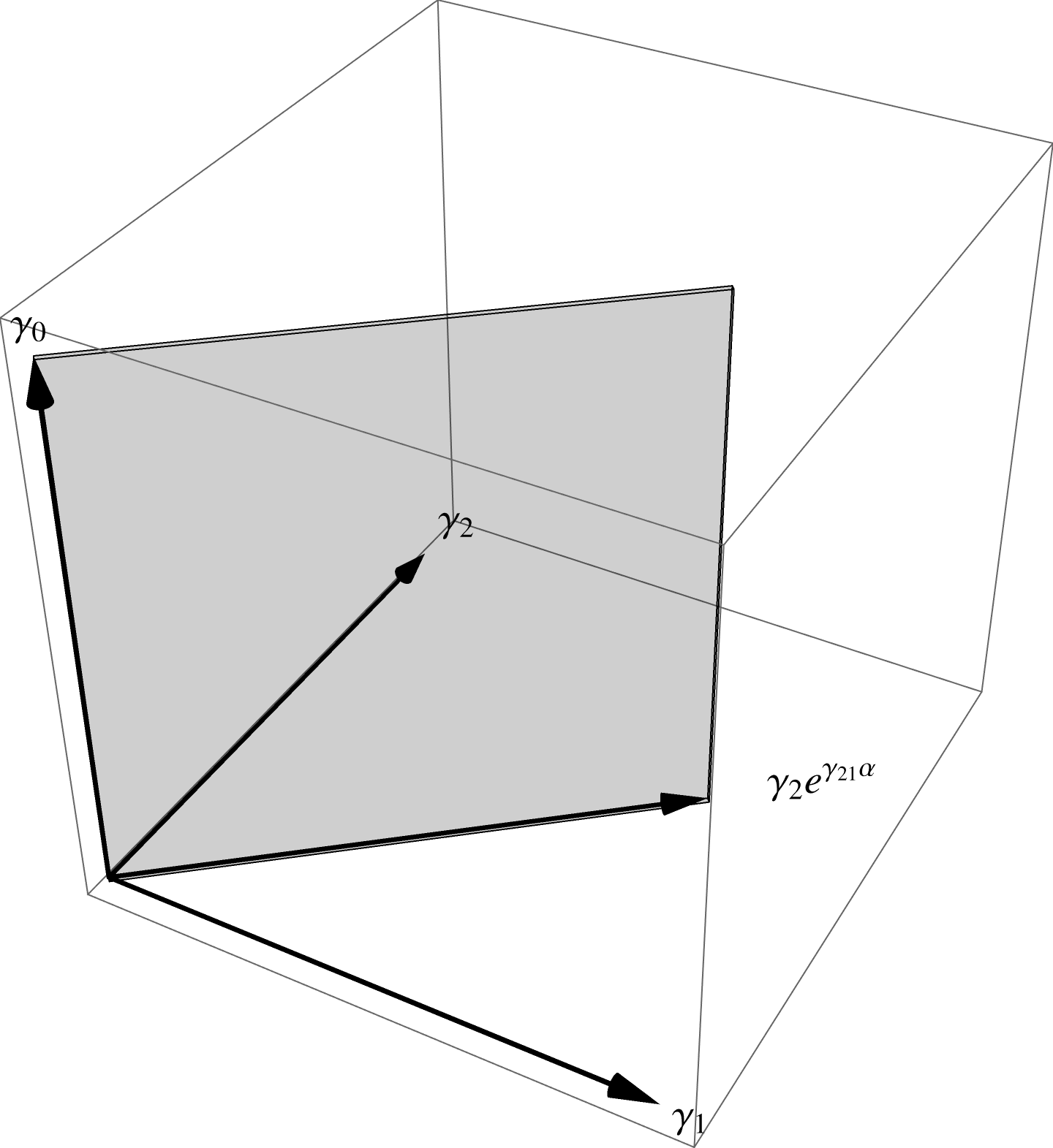
Because \( F \) and \( G \) were both vectors, the resulting integral could only have been a multivector with grades 0,2,4. As it happens, there were no scalar nor pseudoscalar grades in the end result, and we ended up with the spacetime plane between \( \gamma_0 \), and \( \gamma_2 e^{\gamma_{21}\alpha} \), which are rotations of \(\gamma_2\) in the x,y plane. This is illustrated in fig. 1 (omitting scale and sign factors.)

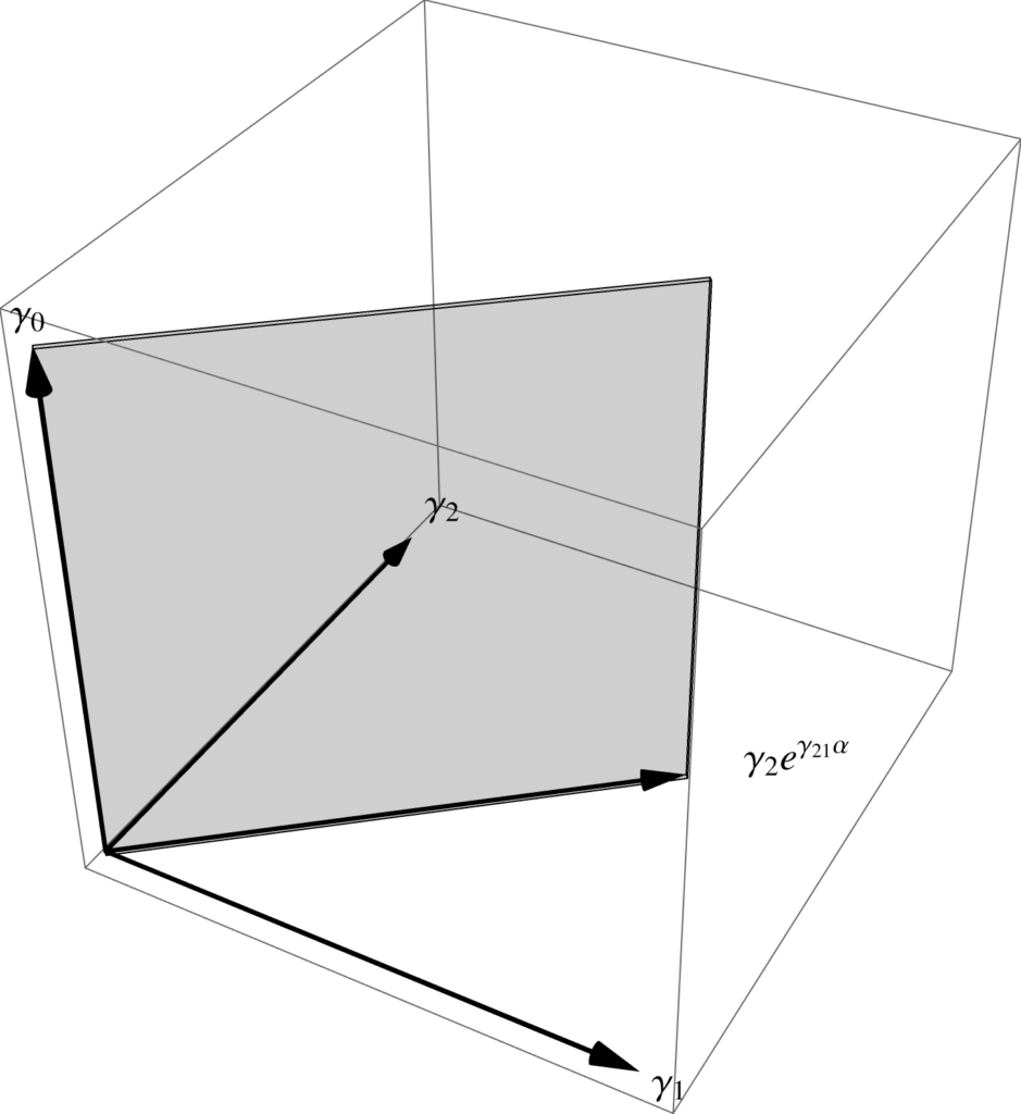
fig. 1. Spacetime plane.

Fundamental theorem for surfaces.

For line integrals we saw that \( d\Bx \cdot \grad = \gpgradezero{ d\Bx \partial } \), and obtained the fundamental theorem for multivector line integrals by omitting the grade selection and using the multivector operator \( d\Bx \partial \) in the integrand directly. We have the same situation for surface integrals. In particular, we know that the \(\mathbb{R}^3\) Stokes theorem can be expressed in terms of \( d^2 \Bx \cdot \spacegrad \)

Problem: GA form of 3D Stokes’ theorem integrand.

Given an \(\mathbb{R}^3\) vector field \( \Bf \), show that
\begin{equation}\label{eqn:relativisticSurface:180}
\int dA \ncap \cdot \lr{ \spacegrad \cross \Bf }
=
-\int \lr{d^2\Bx \cdot \spacegrad } \cdot \Bf.
\end{equation}

Answer

Let \( d^2 \Bx = I \ncap dA \), implicitly fixing the relative orientation of the bivector area element compared to the chosen surface normal direction.
\begin{equation}\label{eqn:relativisticSurface:200}
\begin{aligned}
\int \lr{d^2\Bx \cdot \spacegrad } \cdot \Bf
&=
\int dA \gpgradeone{I \ncap \spacegrad } \cdot \Bf \\
&=
\int dA \lr{ I \lr{ \ncap \wedge \spacegrad} } \cdot \Bf \\
&=
\int dA \gpgradezero{ I^2 \lr{ \ncap \cross \spacegrad} \Bf } \\
&=
-\int dA \lr{ \ncap \cross \spacegrad} \cdot \Bf \\
&=
-\int dA \ncap \cdot \lr{ \spacegrad \cross \Bf }.
\end{aligned}
\end{equation}

The moral of the story is that the conventional dual form of the \(\mathbb{R}^3\) Stokes’ theorem can be written directly by projecting the gradient onto the surface area element. Geometrically, this projection operation has a rotational effect as well, since for bivector \( B \), and vector \( x \), the bivector-vector dot product \( B \cdot x \) is the component of \( x \) that lies in the plane \( B \wedge x = 0 \), but also rotated 90 degrees.

For multivector integration, we do not want an integral operator that includes such dot products. In the line integral case, we were able to achieve the same projective operation by using vector derivative instead of a dot product, and can do the same for the surface integral case. In particular

Theorem 1.1: Projection of gradient onto the tangent space.

Given a curvilinear representation of the gradient with respect to parameters \( u^0, u^1, u^2, u^3 \)
\begin{equation*}
\grad = \sum_\mu \Bx^\mu \PD{u^\mu}{},
\end{equation*}
the surface projection onto the tangent space associated with any two of those parameters, satisfies
\begin{equation*}
d^2 \Bx \cdot \grad = \gpgradeone{ d^2 \Bx \partial }.
\end{equation*}

Start proof:

Without loss of generality, we may pick \( u^0, u^1 \) as the parameters associated with the tangent space. The area element for the surface is
\begin{equation}\label{eqn:relativisticSurface:100}
d^2 \Bx = \Bx_0 \wedge \Bx_1 \,
du^0 du^1.
\end{equation}
Dotting this with the gradient gives
\begin{equation}\label{eqn:relativisticSurface:120}
\begin{aligned}
d^2 \Bx \cdot \grad
&=
du^0 du^1
\lr{ \Bx_0 \wedge \Bx_1 } \cdot \Bx^\mu \PD{u^\mu}{} \\
&=
du^0 du^1
\lr{
\Bx_0
\lr{\Bx_1 \cdot \Bx^\mu }

\Bx_1
\lr{\Bx_0 \cdot \Bx^\mu }
}
\PD{u^\mu}{} \\
&=
du^0 du^1
\lr{
\Bx_0 \PD{u^1}{}

\Bx_0 \PD{u^1}{}
}.
\end{aligned}
\end{equation}
On the other hand, the vector derivative for this surface is
\begin{equation}\label{eqn:relativisticSurface:140}
\partial
=
\Bx^0 \PD{u^0}{}
+
\Bx^1 \PD{u^1}{},
\end{equation}
so
\begin{equation}\label{eqn:relativisticSurface:160}
\begin{aligned}
\gpgradeone{d^2 \Bx \partial}
&=
du^0 du^1\,
\lr{ \Bx_0 \wedge \Bx_1 } \cdot
\lr{
\Bx^0 \PD{u^0}{}
+
\Bx^1 \PD{u^1}{}
} \\
&=
du^0 du^1
\lr{
\Bx_0 \PD{u^1}{}

\Bx_1 \PD{u^0}{}
}.
\end{aligned}
\end{equation}

End proof.

We now want to formulate the geometric algebra form of the fundamental theorem for surface integrals.

Theorem 1.2: Fundamental theorem for surface integrals.

Given multivector functions \( F, G \), and surface area element \( d^2 \Bx = \lr{ \Bx_u \wedge \Bx_v }\, du dv \), associated with a two parameter curve \( x(u,v) \), then
\begin{equation*}
\int_S F d^2\Bx \lrpartial G = \int_{\partial S} F d^1\Bx G,
\end{equation*}
where \( S \) is the integration surface, and \( \partial S \) designates its boundary, and the line integral on the RHS is really short hand for
\begin{equation*}
\int
\evalbar{ \lr{ F (-d\Bx_v) G } }{\Delta u}
+
\int
\evalbar{ \lr{ F (d\Bx_u) G } }{\Delta v},
\end{equation*}
which is a line integral that traverses the boundary of the surface with the opposite orientation to the circulation of the area element.

Start proof:

The vector derivative for this surface is
\begin{equation}\label{eqn:relativisticSurface:220}
\partial =
\Bx^u \PD{u}{}
+
\Bx^v \PD{v}{},
\end{equation}
so
\begin{equation}\label{eqn:relativisticSurface:240}
F d^2\Bx \lrpartial G
=
\PD{u}{} \lr{ F d^2\Bx\, \Bx^u G }
+
\PD{v}{} \lr{ F d^2\Bx\, \Bx^v G },
\end{equation}
where \( d^2\Bx\, \Bx^u \) is held constant with respect to \( u \), and \( d^2\Bx\, \Bx^v \) is held constant with respect to \( v \) (since the partials of the vector derivative act on \( F, G \), but not on the area element, nor on the reciprocal vectors of \( \lrpartial \) itself.) Note that
\begin{equation}\label{eqn:relativisticSurface:260}
d^2\Bx \wedge \Bx^u
=
du dv\, \lr{ \Bx_u \wedge \Bx_v } \wedge \Bx^u = 0,
\end{equation}
since \( \Bx^u \in sectionpan \setlr{ \Bx_u\, \Bx_v } \), so
\begin{equation}\label{eqn:relativisticSurface:280}
\begin{aligned}
d^2\Bx\, \Bx^u
&=
d^2\Bx \cdot \Bx^u
+
d^2\Bx \wedge \Bx^u \\
&=
d^2\Bx \cdot \Bx^u \\
&=
du dv\, \lr{ \Bx_u \wedge \Bx_v } \cdot \Bx^u \\
&=
-du dv\, \Bx_v.
\end{aligned}
\end{equation}
Similarly
\begin{equation}\label{eqn:relativisticSurface:300}
\begin{aligned}
d^2\Bx\, \Bx^v
&=
d^2\Bx \cdot \Bx^v \\
&=
du dv\, \lr{ \Bx_u \wedge \Bx_v } \cdot \Bx^v \\
&=
du dv\, \Bx_u.
\end{aligned}
\end{equation}
This leaves us with
\begin{equation}\label{eqn:relativisticSurface:320}
F d^2\Bx \lrpartial G
=
-du dv\,
\PD{u}{} \lr{ F \Bx_v G }
+
du dv\,
\PD{v}{} \lr{ F \Bx_u G },
\end{equation}
where \( \Bx_v, \Bx_u \) are held constant with respect to \( u,v \) respectively. Fortuitously, this constant condition can be dropped, since the antisymmetry of the wedge in the area element results in perfect cancellation. If these line elements are not held constant then
\begin{equation}\label{eqn:relativisticSurface:340}
\PD{u}{} \lr{ F \Bx_v G }

\PD{v}{} \lr{ F \Bx_u G }
=
F \lr{
\PD{v}{\Bx_u}

\PD{u}{\Bx_v}
} G
+
\lr{
\PD{u}{F} \Bx_v G
+
F \Bx_v \PD{u}{G}
}
+
\lr{
\PD{v}{F} \Bx_u G
+
F \Bx_u \PD{v}{G}
}
,
\end{equation}
but the mixed partial contribution is zero
\begin{equation}\label{eqn:relativisticSurface:360}
\begin{aligned}
\PD{v}{\Bx_u}

\PD{u}{\Bx_v}
&=
\PD{v}{} \PD{u}{x}

\PD{u}{} \PD{v}{x} \\
&=
0,
\end{aligned}
\end{equation}
by equality of mixed partials. We have two perfect differentials, and can evaluate each of these integrals
\begin{equation}\label{eqn:relativisticSurface:380}
\begin{aligned}
\int F d^2\Bx \lrpartial G
&=
-\int
du dv\,
\PD{u}{} \lr{ F \Bx_v G }
+
\int
du dv\,
\PD{v}{} \lr{ F \Bx_u G } \\
&=
-\int
dv\,
\evalbar{ \lr{ F \Bx_v G } }{\Delta u}
+
\int
du\,
\evalbar{ \lr{ F \Bx_u G } }{\Delta v} \\
&=
\int
\evalbar{ \lr{ F (-d\Bx_v) G } }{\Delta u}
+
\int
\evalbar{ \lr{ F (d\Bx_u) G } }{\Delta v}.
\end{aligned}
\end{equation}
We use the shorthand \( d^1 \Bx = d\Bx_u – d\Bx_v \) to write
\begin{equation}\label{eqn:relativisticSurface:400}
\int_S F d^2\Bx \lrpartial G = \int_{\partial S} F d^1\Bx G,
\end{equation}
with the understanding that this is really instructions to evaluate the line integrals in the last step of \ref{eqn:relativisticSurface:380}.

End proof.

Problem: Integration in the t,y plane.

Let \( x(t,y) = c t \gamma_0 + y \gamma_2 \). Write out both sides of the fundamental theorem explicitly.

Answer

Let’s designate the tangent basis vectors as
\begin{equation}\label{eqn:relativisticSurface:420}
\Bx_0 = \PD{t}{x} = c \gamma_0,
\end{equation}
and
\begin{equation}\label{eqn:relativisticSurface:440}
\Bx_2 = \PD{y}{x} = \gamma_2,
\end{equation}
so the vector derivative is
\begin{equation}\label{eqn:relativisticSurface:460}
\partial
= \inv{c} \gamma^0 \PD{t}{}
+ \gamma^2 \PD{y}{},
\end{equation}
and the area element is
\begin{equation}\label{eqn:relativisticSurface:480}
d^2 \Bx = c \gamma_0 \gamma_2.
\end{equation}
The fundamental theorem of surface integrals is just a statement that
\begin{equation}\label{eqn:relativisticSurface:500}
\int_{t_0}^{t_1} c dt
\int_{y_0}^{y_1} dy
F \gamma_0 \gamma_2 \lr{
\inv{c} \gamma^0 \PD{t}{}
+ \gamma^2 \PD{y}{}
} G
=
\int F \lr{ c \gamma_0 dt – \gamma_2 dy } G,
\end{equation}
where the RHS, when stated explicitly, really means
\begin{equation}\label{eqn:relativisticSurface:520}
\begin{aligned}
\int &F \lr{ c \gamma_0 dt – \gamma_2 dy } G
=
\int_{t_0}^{t_1} c dt \lr{ F(t,y_1) \gamma_0 G(t, y_1) – F(t,y_0) \gamma_0 G(t, y_0) } \\
&\qquad –
\int_{y_0}^{y_1} dy \lr{ F(t_1,y) \gamma_2 G(t_1, y) – F(t_0,y) \gamma_0 G(t_0, y) }.
\end{aligned}
\end{equation}
In this particular case, since \( \Bx_0 = c \gamma_0, \Bx_2 = \gamma_2 \) are both constant functions that depend on neither \( t \) nor \( y \), it is easy to derive the full expansion of \ref{eqn:relativisticSurface:520} directly from the LHS of \ref{eqn:relativisticSurface:500}.

Problem: A cylindrical hyperbolic surface.

Generalizing the example surface integral from \ref{eqn:relativisticSurface:40}, let
\begin{equation}\label{eqn:relativisticSurface:540}
x(\rho, \alpha) = \rho e^{-\vcap \alpha/2} x(0,1) e^{\vcap \alpha/2},
\end{equation}
where \( \rho \) is a scalar, and \( \vcap = \cos\theta_k\gamma_{k0} \) is a unit spatial bivector, and \( \cos\theta_k \) are direction cosines of that vector. This is a composite transformation, where the \( \alpha \) variation boosts the \( x(0,1) \) four-vector, and the \( \rho \) parameter contracts or increases the magnitude of this vector, resulting in \( x \) spanning a hyperbolic region of spacetime.

Compute the tangent and reciprocal basis, the area element for the surface, and explicitly state both sides of the fundamental theorem.

Answer

For the tangent basis vectors we have
\begin{equation}\label{eqn:relativisticSurface:560}
\Bx_\rho = \PD{\rho}{x} =
e^{-\vcap \alpha/2} x(0,1) e^{\vcap \alpha/2} = \frac{x}{\rho},
\end{equation}
and
\begin{equation}\label{eqn:relativisticSurface:580}
\Bx_\alpha = \PD{\alpha}{x} =
\lr{-\vcap/2} x
+
x \lr{ \vcap/2 }
=
x \cdot \vcap.
\end{equation}
These vectors \( \Bx_\rho, \Bx_\alpha \) are orthogonal, as \( x \cdot \vcap \) is the projection of \( x \) onto the spacetime plane \( x \wedge \vcap = 0 \), but rotated so that \( x \cdot \lr{ x \cdot \vcap } = 0 \). Because of this orthogonality, the vector derivative for this tangent space is
\begin{equation}\label{eqn:relativisticSurface:600}
\partial =
\inv{x \cdot \vcap} \PD{\alpha}{}
+
\frac{\rho}{x}
\PD{\rho}{}
.
\end{equation}
The area element is
\begin{equation}\label{eqn:relativisticSurface:620}
\begin{aligned}
d^2 \Bx
&=
d\rho d\alpha\,
\frac{x}{\rho} \wedge \lr{ x \cdot \vcap } \\
&=
\inv{\rho} d\rho d\alpha\,
x \lr{ x \cdot \vcap }
.
\end{aligned}
\end{equation}
The full statement of the fundamental theorem for this surface is
\begin{equation}\label{eqn:relativisticSurface:640}
\int_S
d\rho d\alpha\,
F
\lr{
\inv{\rho} x \lr{ x \cdot \vcap }
}
\lr{
\inv{x \cdot \vcap} \PD{\alpha}{}
+
\frac{\rho}{x}
\PD{\rho}{}
}
G
=
\int_{\partial S}
F \lr{ d\rho \frac{x}{\rho} – d\alpha \lr{ x \cdot \vcap } } G.
\end{equation}
As in the previous example, due to the orthogonality of the tangent basis vectors, it’s easy to show find the RHS directly from the LHS.

Problem: Simple example with non-orthogonal tangent space basis vectors.

Let \( x(u,v) = u a + v b \), where \( u,v \) are scalar parameters, and \( a, b \) are non-null and non-colinear constant four-vectors. Write out the fundamental theorem for surfaces with respect to this parameterization.

Answer

The tangent basis vectors are just \( \Bx_u = a, \Bx_v = b \), with reciprocals
\begin{equation}\label{eqn:relativisticSurface:660}
\Bx^u = \Bx_v \cdot \inv{ \Bx_u \wedge \Bx_v } = b \cdot \inv{ a \wedge b },
\end{equation}
and
\begin{equation}\label{eqn:relativisticSurface:680}
\Bx^v = -\Bx_u \cdot \inv{ \Bx_u \wedge \Bx_v } = -a \cdot \inv{ a \wedge b }.
\end{equation}
The fundamental theorem, with respect to this surface, when written out explicitly takes the form
\begin{equation}\label{eqn:relativisticSurface:700}
\int F \, du dv\, \lr{ a \wedge b } \inv{ a \wedge b } \cdot \lr{ a \PD{u}{} – b \PD{v}{} } G
=
\int F \lr{ a du – b dv } G.
\end{equation}
This is a good example to illustrate the geometry of the line integral circulation.
Suppose that we are integrating over \( u \in [0,1], v \in [0,1] \). In this case, the line integral really means
\begin{equation}\label{eqn:relativisticSurface:720}
\begin{aligned}
\int &F \lr{ a du – b dv } G
=
+
\int F(u,1) (+a du) G(u,1)
+
\int F(u,0) (-a du) G(u,0) \\
&\quad+
\int F(1,v) (-b dv) G(1,v)
+
\int F(0,v) (+b dv) G(0,v),
\end{aligned}
\end{equation}
which is a path around the spacetime parallelogram spanned by \( u, v \), as illustrated in fig. 1, which illustrates the orientation of the bivector area element with the arrows around the exterior of the parallelogram: \( 0 \rightarrow a \rightarrow a + b \rightarrow b \rightarrow 0 \).

fig. 2. Line integral orientation.

Fundamental theorem of geometric calculus for line integrals (relativistic.)

December 16, 2020 math and physics play , , , , , , , , , , , , , , , , , , , , , , , , , , ,

[This post is best viewed in PDF form, due to latex elements that I could not format with wordpress mathjax.]

Background for this particular post can be found in

  1. Curvilinear coordinates and gradient in spacetime, and reciprocal frames, and
  2. Lorentz transformations in Space Time Algebra (STA)
  3. A couple more reciprocal frame examples.

Motivation.

I’ve been slowly working my way towards a statement of the fundamental theorem of integral calculus, where the functions being integrated are elements of the Dirac algebra (space time multivectors in the geometric algebra parlance.)

This is interesting because we want to be able to do line, surface, 3-volume and 4-volume space time integrals. We have many \(\mathbb{R}^3\) integral theorems
\begin{equation}\label{eqn:fundamentalTheoremOfGC:40a}
\int_A^B d\Bl \cdot \spacegrad f = f(B) – f(A),
\end{equation}
\begin{equation}\label{eqn:fundamentalTheoremOfGC:60a}
\int_S dA\, \ncap \cross \spacegrad f = \int_{\partial S} d\Bx\, f,
\end{equation}
\begin{equation}\label{eqn:fundamentalTheoremOfGC:80a}
\int_S dA\, \ncap \cdot \lr{ \spacegrad \cross \Bf} = \int_{\partial S} d\Bx \cdot \Bf,
\end{equation}
\begin{equation}\label{eqn:fundamentalTheoremOfGC:100a}
\int_S dx dy \lr{ \PD{y}{P} – \PD{x}{Q} }
=
\int_{\partial S} P dx + Q dy,
\end{equation}
\begin{equation}\label{eqn:fundamentalTheoremOfGC:120a}
\int_V dV\, \spacegrad f = \int_{\partial V} dA\, \ncap f,
\end{equation}
\begin{equation}\label{eqn:fundamentalTheoremOfGC:140a}
\int_V dV\, \spacegrad \cross \Bf = \int_{\partial V} dA\, \ncap \cross \Bf,
\end{equation}
\begin{equation}\label{eqn:fundamentalTheoremOfGC:160a}
\int_V dV\, \spacegrad \cdot \Bf = \int_{\partial V} dA\, \ncap \cdot \Bf,
\end{equation}
and want to know how to generalize these to four dimensions and also make sure that we are handling the relativistic mixed signature correctly. If our starting point was the mess of equations above, we’d be in trouble, since it is not obvious how these generalize. All the theorems with unit normals have to be handled completely differently in four dimensions since we don’t have a unique normal to any given spacetime plane.
What comes to our rescue is the Fundamental Theorem of Geometric Calculus (FTGC), which has the form
\begin{equation}\label{eqn:fundamentalTheoremOfGC:40}
\int F d^n \Bx\, \lrpartial G = \int F d^{n-1} \Bx\, G,
\end{equation}
where \(F,G\) are multivectors functions (i.e. sums of products of vectors.) We’ve seen ([2], [1]) that all the identities above are special cases of the fundamental theorem.

Do we need any special care to state the FTGC correctly for our relativistic case? It turns out that the answer is no! Tangent and reciprocal frame vectors do all the heavy lifting, and we can use the fundamental theorem as is, even in our mixed signature space. The only real change that we need to make is use spacetime gradient and vector derivative operators instead of their spatial equivalents. We will see how this works below. Note that instead of starting with \ref{eqn:fundamentalTheoremOfGC:40} directly, I will attempt to build up to that point in a progressive fashion that is hopefully does not require the reader to make too many unjustified mental leaps.

Multivector line integrals.

We want to define multivector line integrals to start with. Recall that in \(\mathbb{R}^3\) we would say that for scalar functions \( f\), the integral
\begin{equation}\label{eqn:fundamentalTheoremOfGC:180b}
\int d\Bx\, f = \int f d\Bx,
\end{equation}
is a line integral. Also, for vector functions \( \Bf \) we call
\begin{equation}\label{eqn:fundamentalTheoremOfGC:200}
\int d\Bx \cdot \Bf = \inv{2} \int d\Bx\, \Bf + \Bf d\Bx.
\end{equation}
a line integral. In order to generalize line integrals to multivector functions, we will allow our multivector functions to be placed on either or both sides of the differential.

Definition 1.1: Line integral.

Given a single variable parameterization \( x = x(u) \), we write \( d^1\Bx = \Bx_u du \), and call
\begin{equation}\label{eqn:fundamentalTheoremOfGC:220a}
\int F d^1\Bx\, G,
\end{equation}
a line integral, where \( F,G \) are arbitrary multivector functions.

We must be careful not to reorder any of the factors in the integrand, since the differential may not commute with either \( F \) or \( G \). Here is a simple example where the integrand has a product of a vector and differential.

Problem: Circular parameterization.

Given a circular parameterization \( x(\theta) = \gamma_1 e^{-i\theta} \), where \( i = \gamma_1 \gamma_2 \), the unit bivector for the \(x,y\) plane. Compute the line integral
\begin{equation}\label{eqn:fundamentalTheoremOfGC:100}
\int_0^{\pi/4} F(\theta)\, d^1 \Bx\, G(\theta),
\end{equation}
where \( F(\theta) = \Bx^\theta + \gamma_3 + \gamma_1 \gamma_0 \) is a multivector valued function, and \( G(\theta) = \gamma_0 \) is vector valued.

Answer

The tangent vector for the curve is
\begin{equation}\label{eqn:fundamentalTheoremOfGC:60}
\Bx_\theta
= -\gamma_1 \gamma_1 \gamma_2 e^{-i\theta}
= \gamma_2 e^{-i\theta},
\end{equation}
with reciprocal vector \( \Bx^\theta = e^{i \theta} \gamma^2 \). The differential element is \( d^1 \Bx = \gamma_2 e^{-i\theta} d\theta \), so the integrand is
\begin{equation}\label{eqn:fundamentalTheoremOfGC:80}
\begin{aligned}
\int_0^{\pi/4} \lr{ \Bx^\theta + \gamma_3 + \gamma_1 \gamma_0 } d^1 \Bx\, \gamma_0
&=
\int_0^{\pi/4} \lr{ e^{i\theta} \gamma^2 + \gamma_3 + \gamma_1 \gamma_0 } \gamma_2 e^{-i\theta} d\theta\, \gamma_0 \\
&=
\frac{\pi}{4} \gamma_0 + \lr{ \gamma_{32} + \gamma_{102} } \inv{-i} \lr{ e^{-i\pi/4} – 1 } \gamma_0 \\
&=
\frac{\pi}{4} \gamma_0 + \inv{\sqrt{2}} \lr{ \gamma_{32} + \gamma_{102} } \gamma_{120} \lr{ 1 – \gamma_{12} } \\
&=
\frac{\pi}{4} \gamma_0 + \inv{\sqrt{2}} \lr{ \gamma_{310} + 1 } \lr{ 1 – \gamma_{12} }.
\end{aligned}
\end{equation}
Observe how care is required not to reorder any terms. This particular end result is a multivector with scalar, vector, bivector, and trivector grades, but no pseudoscalar component. The grades in the end result depend on both the function in the integrand and on the path. For example, had we integrated all the way around the circle, the end result would have been the vector \( 2 \pi \gamma_0 \) (i.e. a \( \gamma_0 \) weighted unit circle circumference), as all the other grades would have been killed by the complex exponential integrated over a full period.

Problem: Line integral for boosted time direction vector.

Let \( x = e^{\vcap \alpha/2} \gamma_0 e^{-\vcap \alpha/2} \) represent the spacetime curve of all the boosts of \( \gamma_0 \) along a specific velocity direction vector, where \( \vcap = (v \wedge \gamma_0)/\Norm{v \wedge \gamma_0} \) is a unit spatial bivector for any constant vector \( v \). Compute the line integral
\begin{equation}\label{eqn:fundamentalTheoremOfGC:240}
\int x\, d^1 \Bx.
\end{equation}

Answer

Observe that \( \vcap \) and \( \gamma_0 \) anticommute, so we may write our boost as a one sided exponential
\begin{equation}\label{eqn:fundamentalTheoremOfGC:260}
x(\alpha) = \gamma_0 e^{-\vcap \alpha} = e^{\vcap \alpha} \gamma_0 = \lr{ \cosh\alpha + \vcap \sinh\alpha } \gamma_0.
\end{equation}
The tangent vector is just
\begin{equation}\label{eqn:fundamentalTheoremOfGC:280}
\Bx_\alpha = \PD{\alpha}{x} = e^{\vcap\alpha} \vcap \gamma_0.
\end{equation}
Let’s get a bit of intuition about the nature of this vector. It’s square is
\begin{equation}\label{eqn:fundamentalTheoremOfGC:300}
\begin{aligned}
\Bx_\alpha^2
&=
e^{\vcap\alpha} \vcap \gamma_0
e^{\vcap\alpha} \vcap \gamma_0 \\
&=
-e^{\vcap\alpha} \vcap e^{-\vcap\alpha} \vcap (\gamma_0)^2 \\
&=
-1,
\end{aligned}
\end{equation}
so we see that the tangent vector is a spacelike unit vector. As the vector representing points on the curve is necessarily timelike (due to Lorentz invariance), these two must be orthogonal at all points. Let’s confirm this algebraically
\begin{equation}\label{eqn:fundamentalTheoremOfGC:320}
\begin{aligned}
x \cdot \Bx_\alpha
&=
\gpgradezero{ e^{\vcap \alpha} \gamma_0 e^{\vcap \alpha} \vcap \gamma_0 } \\
&=
\gpgradezero{ e^{-\vcap \alpha} e^{\vcap \alpha} \vcap (\gamma_0)^2 } \\
&=
\gpgradezero{ \vcap } \\
&= 0.
\end{aligned}
\end{equation}
Here we used \( e^{\vcap \alpha} \gamma_0 = \gamma_0 e^{-\vcap \alpha} \), and \( \gpgradezero{A B} = \gpgradezero{B A} \). Geometrically, we have the curious fact that the direction vectors to points on the curve are perpendicular (with respect to our relativistic dot product) to the tangent vectors on the curve, as illustrated in fig. 1.

fig. 1. Tangent perpendicularity in mixed metric.

Perfect differentials.

Having seen a couple examples of multivector line integrals, let’s now move on to figure out the structure of a line integral that has a “perfect” differential integrand. We can take a hint from the \(\mathbb{R}^3\) vector result that we already know, namely
\begin{equation}\label{eqn:fundamentalTheoremOfGC:120}
\int_A^B d\Bl \cdot \spacegrad f = f(B) – f(A).
\end{equation}
It seems reasonable to guess that the relativistic generalization of this is
\begin{equation}\label{eqn:fundamentalTheoremOfGC:140}
\int_A^B dx \cdot \grad f = f(B) – f(A).
\end{equation}
Let’s check that, by expanding in coordinates
\begin{equation}\label{eqn:fundamentalTheoremOfGC:160}
\begin{aligned}
\int_A^B dx \cdot \grad f
&=
\int_A^B d\tau \frac{dx^\mu}{d\tau} \partial_\mu f \\
&=
\int_A^B d\tau \frac{dx^\mu}{d\tau} \PD{x^\mu}{f} \\
&=
\int_A^B d\tau \frac{df}{d\tau} \\
&=
f(B) – f(A).
\end{aligned}
\end{equation}
If we drop the dot product, will we have such a nice result? Let’s see:
\begin{equation}\label{eqn:fundamentalTheoremOfGC:180}
\begin{aligned}
\int_A^B dx \grad f
&=
\int_A^B d\tau \frac{dx^\mu}{d\tau} \gamma_\mu \gamma^\nu \partial_\nu f \\
&=
\int_A^B d\tau \frac{dx^\mu}{d\tau} \PD{x^\mu}{f}
+
\int_A^B
d\tau
\sum_{\mu \ne \nu} \gamma_\mu \gamma^\nu
\frac{dx^\mu}{d\tau} \PD{x^\nu}{f}.
\end{aligned}
\end{equation}
This scalar component of this integrand is a perfect differential, but the bivector part of the integrand is a complete mess, that we have no hope of generally integrating. It happens that if we consider one of the simplest parameterization examples, we can get a strong hint of how to generalize the differential operator to one that ends up providing a perfect differential. In particular, let’s integrate over a linear constant path, such as \( x(\tau) = \tau \gamma_0 \). For this path, we have
\begin{equation}\label{eqn:fundamentalTheoremOfGC:200a}
\begin{aligned}
\int_A^B dx \grad f
&=
\int_A^B \gamma_0 d\tau \lr{
\gamma^0 \partial_0 +
\gamma^1 \partial_1 +
\gamma^2 \partial_2 +
\gamma^3 \partial_3 } f \\
&=
\int_A^B d\tau \lr{
\PD{\tau}{f} +
\gamma_0 \gamma^1 \PD{x^1}{f} +
\gamma_0 \gamma^2 \PD{x^2}{f} +
\gamma_0 \gamma^3 \PD{x^3}{f}
}.
\end{aligned}
\end{equation}
Just because the path does not have any \( x^1, x^2, x^3 \) component dependencies does not mean that these last three partials are neccessarily zero. For example \( f = f(x(\tau)) = \lr{ x^0 }^2 \gamma_0 + x^1 \gamma_1 \) will have a non-zero contribution from the \( \partial_1 \) operator. In that particular case, we can easily integrate \( f \), but we have to know the specifics of the function to do the integral. However, if we had a differential operator that did not include any component off the integration path, we would ahve a perfect differential. That is, if we were to replace the gradient with the projection of the gradient onto the tangent space, we would have a perfect differential. We see that the function of the dot product in \ref{eqn:fundamentalTheoremOfGC:140} has the same effect, as it rejects any component of the gradient that does not lie on the tangent space.

Definition 1.2: Vector derivative.

Given a spacetime manifold parameterized by \( x = x(u^0, \cdots u^{N-1}) \), with tangent vectors \( \Bx_\mu = \PDi{u^\mu}{x} \), and reciprocal vectors \( \Bx^\mu \in \textrm{Span}\setlr{\Bx_\nu} \), such that \( \Bx^\mu \cdot \Bx_\nu = {\delta^\mu}_\nu \), the vector derivative is defined as
\begin{equation}\label{eqn:fundamentalTheoremOfGC:240a}
\partial = \sum_{\mu = 0}^{N-1} \Bx^\mu \PD{u^\mu}{}.
\end{equation}
Observe that if this is a full parameterization of the space (\(N = 4\)), then the vector derivative is identical to the gradient. The vector derivative is the projection of the gradient onto the tangent space at the point of evaluation.Furthermore, we designate \( \lrpartial \) as the vector derivative allowed to act bidirectionally, as follows
\begin{equation}\label{eqn:fundamentalTheoremOfGC:260a}
R \lrpartial S
=
R \Bx^\mu \PD{u^\mu}{S}
+
\PD{u^\mu}{R} \Bx^\mu S,
\end{equation}
where \( R, S \) are multivectors, and summation convention is implied. In this bidirectional action,
the vector factors of the vector derivative must stay in place (as they do not neccessarily commute with \( R,S\)), but the derivative operators apply in a chain rule like fashion to both functions.

Noting that \( \Bx_u \cdot \grad = \Bx_u \cdot \partial \), we may rewrite the scalar line integral identity \ref{eqn:fundamentalTheoremOfGC:140} as
\begin{equation}\label{eqn:fundamentalTheoremOfGC:220}
\int_A^B dx \cdot \partial f = f(B) – f(A).
\end{equation}
However, as our example hinted at, the fundamental theorem for line integrals has a multivector generalization that does not rely on a dot product to do the tangent space filtering, and is more powerful. That generalization has the following form.

Theorem 1.1: Fundamental theorem for line integrals.

Given multivector functions \( F, G \), and a single parameter curve \( x(u) \) with line element \( d^1 \Bx = \Bx_u du \), then
\begin{equation}\label{eqn:fundamentalTheoremOfGC:280a}
\int_A^B F d^1\Bx \lrpartial G = F(B) G(B) – F(A) G(A).
\end{equation}

Start proof:

Writing out the integrand explicitly, we find
\begin{equation}\label{eqn:fundamentalTheoremOfGC:340}
\int_A^B F d^1\Bx \lrpartial G
=
\int_A^B \lr{
\PD{\alpha}{F} d\alpha\, \Bx_\alpha \Bx^\alpha G
+
F d\alpha\, \Bx_\alpha \Bx^\alpha \PD{\alpha}{G }
}
\end{equation}
However for a single parameter curve, we have \( \Bx^\alpha = 1/\Bx_\alpha \), so we are left with
\begin{equation}\label{eqn:fundamentalTheoremOfGC:360}
\begin{aligned}
\int_A^B F d^1\Bx \lrpartial G
&=
\int_A^B d\alpha\, \PD{\alpha}{(F G)} \\
&=
\evalbar{F G}{B}

\evalbar{F G}{A}.
\end{aligned}
\end{equation}

End proof.

More to come.

In the next installment we will explore surface integrals in spacetime, and the generalization of the fundamental theorem to multivector space time integrals.

References

[1] Peeter Joot. Geometric Algebra for Electrical Engineers. Kindle Direct Publishing, 2019.

[2] A. Macdonald. Vector and Geometric Calculus. CreateSpace Independent Publishing Platform, 2012.

New version of Geometric Algebra for Electrical Engineers posted.

September 24, 2018 math and physics play , , , , ,


A new version of Geometric Algebra for Electrical Engineers (V0.1.8) is now posted.  This fixes a number of issues in Chapter II on geometric calculus.  In particular, I had confused definitions of line, area, and volume integrals that were really the application of the fundamental theorem to such integrals.  This is now fixed, and the whole chapter is generally improved and clarified.

Helmholtz theorem

October 1, 2016 math and physics play , , , , , , , , , , , , , ,

[Click here for a PDF of this post with nicer formatting]

This is a problem from ece1228. I attempted solutions in a number of ways. One using Geometric Algebra, one devoid of that algebra, and then this method, which combined aspects of both. Of the three methods I tried to obtain this result, this is the most compact and elegant. It does however, require a fair bit of Geometric Algebra knowledge, including the Fundamental Theorem of Geometric Calculus, as detailed in [1], [3] and [2].

Question: Helmholtz theorem

Prove the first Helmholtz’s theorem, i.e. if vector \(\BM\) is defined by its divergence

\begin{equation}\label{eqn:helmholtzDerviationMultivector:20}
\spacegrad \cdot \BM = s
\end{equation}

and its curl
\begin{equation}\label{eqn:helmholtzDerviationMultivector:40}
\spacegrad \cross \BM = \BC
\end{equation}

within a region and its normal component \( \BM_{\textrm{n}} \) over the boundary, then \( \BM \) is
uniquely specified.

Answer

The gradient of the vector \( \BM \) can be written as a single even grade multivector

\begin{equation}\label{eqn:helmholtzDerviationMultivector:60}
\spacegrad \BM
= \spacegrad \cdot \BM + I \spacegrad \cross \BM
= s + I \BC.
\end{equation}

We will use this to attempt to discover the relation between the vector \( \BM \) and its divergence and curl. We can express \( \BM \) at the point of interest as a convolution with the delta function at all other points in space

\begin{equation}\label{eqn:helmholtzDerviationMultivector:80}
\BM(\Bx) = \int_V dV’ \delta(\Bx – \Bx’) \BM(\Bx’).
\end{equation}

The Laplacian representation of the delta function in \R{3} is

\begin{equation}\label{eqn:helmholtzDerviationMultivector:100}
\delta(\Bx – \Bx’) = -\inv{4\pi} \spacegrad^2 \inv{\Abs{\Bx – \Bx’}},
\end{equation}

so \( \BM \) can be represented as the following convolution

\begin{equation}\label{eqn:helmholtzDerviationMultivector:120}
\BM(\Bx) = -\inv{4\pi} \int_V dV’ \spacegrad^2 \inv{\Abs{\Bx – \Bx’}} \BM(\Bx’).
\end{equation}

Using this relation and proceeding with a few applications of the chain rule, plus the fact that \( \spacegrad 1/\Abs{\Bx – \Bx’} = -\spacegrad’ 1/\Abs{\Bx – \Bx’} \), we find

\begin{equation}\label{eqn:helmholtzDerviationMultivector:720}
\begin{aligned}
-4 \pi \BM(\Bx)
&= \int_V dV’ \spacegrad^2 \inv{\Abs{\Bx – \Bx’}} \BM(\Bx’) \\
&= \gpgradeone{\int_V dV’ \spacegrad^2 \inv{\Abs{\Bx – \Bx’}} \BM(\Bx’)} \\
&= -\gpgradeone{\int_V dV’ \spacegrad \lr{ \spacegrad’ \inv{\Abs{\Bx – \Bx’}}} \BM(\Bx’)} \\
&= -\gpgradeone{\spacegrad \int_V dV’ \lr{
\spacegrad’ \frac{\BM(\Bx’)}{\Abs{\Bx – \Bx’}}
-\frac{\spacegrad’ \BM(\Bx’)}{\Abs{\Bx – \Bx’}}
} } \\
&=
-\gpgradeone{\spacegrad \int_{\partial V} dA’
\ncap \frac{\BM(\Bx’)}{\Abs{\Bx – \Bx’}}
}
+\gpgradeone{\spacegrad \int_V dV’
\frac{s(\Bx’) + I\BC(\Bx’)}{\Abs{\Bx – \Bx’}}
} \\
&=
-\gpgradeone{\spacegrad \int_{\partial V} dA’
\ncap \frac{\BM(\Bx’)}{\Abs{\Bx – \Bx’}}
}
+\spacegrad \int_V dV’
\frac{s(\Bx’)}{\Abs{\Bx – \Bx’}}
+\spacegrad \cdot \int_V dV’
\frac{I\BC(\Bx’)}{\Abs{\Bx – \Bx’}}.
\end{aligned}
\end{equation}

By inserting a no-op grade selection operation in the second step, the trivector terms that would show up in subsequent steps are automatically filtered out. This leaves us with a boundary term dependent on the surface and the normal and tangential components of \( \BM \). Added to that is a pair of volume integrals that provide the unique dependence of \( \BM \) on its divergence and curl. When the surface is taken to infinity, which requires \( \Abs{\BM}/\Abs{\Bx – \Bx’} \rightarrow 0 \), then the dependence of \( \BM \) on its divergence and curl is unique.

In order to express final result in traditional vector algebra form, a couple transformations are required. The first is that

\begin{equation}\label{eqn:helmholtzDerviationMultivector:800}
\gpgradeone{ \Ba I \Bb } = I^2 \Ba \cross \Bb = -\Ba \cross \Bb.
\end{equation}

For the grade selection in the boundary integral, note that

\begin{equation}\label{eqn:helmholtzDerviationMultivector:740}
\begin{aligned}
\gpgradeone{ \spacegrad \ncap \BX }
&=
\gpgradeone{ \spacegrad (\ncap \cdot \BX) }
+
\gpgradeone{ \spacegrad (\ncap \wedge \BX) } \\
&=
\spacegrad (\ncap \cdot \BX)
+
\gpgradeone{ \spacegrad I (\ncap \cross \BX) } \\
&=
\spacegrad (\ncap \cdot \BX)

\spacegrad \cross (\ncap \cross \BX).
\end{aligned}
\end{equation}

These give

\begin{equation}\label{eqn:helmholtzDerviationMultivector:721}
\boxed{
\begin{aligned}
\BM(\Bx)
&=
\spacegrad \inv{4\pi} \int_{\partial V} dA’ \ncap \cdot \frac{\BM(\Bx’)}{\Abs{\Bx – \Bx’}}

\spacegrad \cross \inv{4\pi} \int_{\partial V} dA’ \ncap \cross \frac{\BM(\Bx’)}{\Abs{\Bx – \Bx’}} \\
&-\spacegrad \inv{4\pi} \int_V dV’
\frac{s(\Bx’)}{\Abs{\Bx – \Bx’}}
+\spacegrad \cross \inv{4\pi} \int_V dV’
\frac{\BC(\Bx’)}{\Abs{\Bx – \Bx’}}.
\end{aligned}
}
\end{equation}

References

[1] C. Doran and A.N. Lasenby. Geometric algebra for physicists. Cambridge University Press New York, Cambridge, UK, 1st edition, 2003.

[2] A. Macdonald. Vector and Geometric Calculus. CreateSpace Independent Publishing Platform, 2012.

[3] Garret Sobczyk and Omar Le’on S’anchez. Fundamental theorem of calculus. Advances in Applied Clifford Algebras, 21:221–231, 2011. URL https://arxiv.org/abs/0809.4526.