Day: November 10, 2014

ECE1254H Modeling of Multiphysics Systems. Lecture 14: Backward Euler method and trapezoidal methods. Taught by Prof. Piero Triverio

November 10, 2014 ece1254 , , ,

[Click here for a PDF of this post with nicer formatting]

Disclaimer

Peeter’s lecture notes from class. These may be incoherent and rough.

Backward Euler method

Discretized time dependent partial differential equations were seen to have the form

\begin{equation}\label{eqn:multiphysicsL14:20}
G \Bx(t) + C \dot{\Bx}(t) = B \Bu(t),
\end{equation}

where \( G, C, B \) are matrices, and \( \Bu(t) \) is a vector of sources.

The backward Euler method augments \ref{eqn:multiphysicsL14:20} with an initial condition. For a one dimensional system such an initial condition could a zero time specification

\begin{equation}\label{eqn:multiphysicsL14:40}
G x(t) + C \dot{x}(t) = B u(t),
\end{equation}
\begin{equation}\label{eqn:multiphysicsL14:60}
x(0) = x_0
\end{equation}

Discretizing time as in fig. 1.

lecture14Fig1

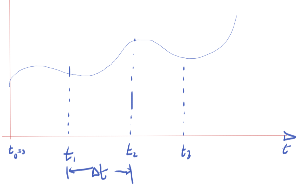
fig. 1. Discretized time

The discrete derivative, using a backward difference, is

\begin{equation}\label{eqn:multiphysicsL14:80}
\dot{x}(t = t_n) \approx \frac{ x_n – x_{n-1} }{\Delta t}
\end{equation}

Evaluating \ref{eqn:multiphysicsL14:40} at \( t = t_n \) is

\begin{equation}\label{eqn:multiphysicsL14:100}
G x_n + C \dot{x}(t = t_n) = B u(t_n),
\end{equation}

or approximately

\begin{equation}\label{eqn:multiphysicsL14:120}
G x_n + C \frac{x_n – x_{n-1}}{\Delta t} = B u(t_n).
\end{equation}

Rearranging

\begin{equation}\label{eqn:multiphysicsL14:140}
\lr{ G + \frac{C}{\Delta t} } x_n = \frac{C}{\Delta t} x_{n-1}
+
B u(t_n).
\end{equation}

Assuming that matrices \( G, C \) are constant, and \( \Delta t \) is fixed, a matrix inversion can be avoided, and a single LU decomposition can be used. For \( N \) sampling points (not counting \( t_0 = 0 \)), \( N \) sets of backward and forward substitutions will be required to compute \( x_1 \) from \( x_0 \), and so forth.

Backwards Euler is an implicit method.

Recall that the forward Euler method gave

\begin{equation}\label{eqn:multiphysicsL14:160}
x_{n+1} =
x_n \lr{ I – C^{-1} \Delta t G }
+ C^{-1} \Delta t B u(t_n)
\end{equation}

This required

  • \( C \) must be invertible.
  • \( C \) must be cheap to invert, perhaps \( C = I \), so that
    \begin{equation}\label{eqn:multiphysicsL14:180}
    x_{n+1} =
    \lr{ I – \Delta t G } x_n
    + \Delta t B u(t_n)
    \end{equation}
  • This is an explicit method
  • This can be cheap but unstable.

Trapezoidal rule (TR)

The derivative can be approximated using an average of the pair of derivatives as illustrated in fig. 2.

lecture14Fig2

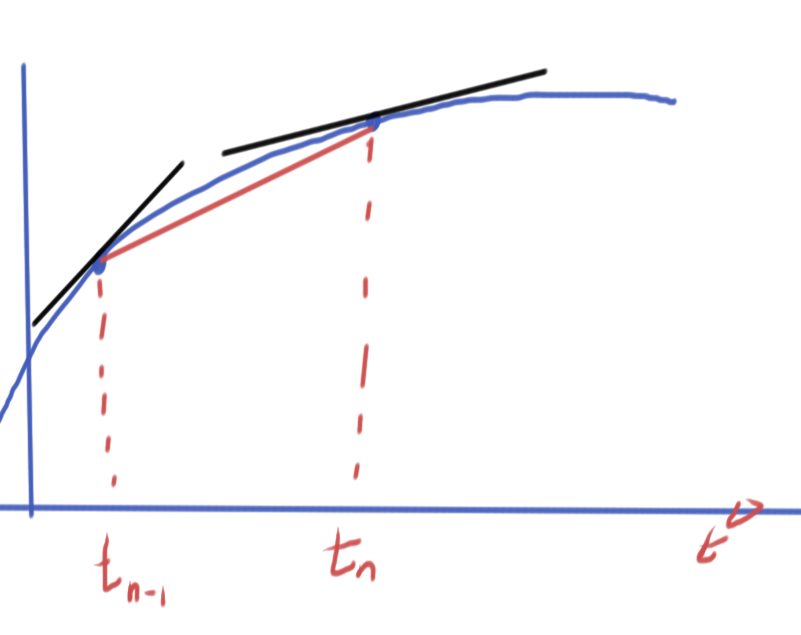
fig. 2. Trapezoidal derivative approximation

\begin{equation}\label{eqn:multiphysicsL14:200}
\frac{x_n – x_{n-1}}{\Delta t} \approx \frac{
\dot{x}(t_{n-1})
+
\dot{x}(t_{n})
}
{2}.
\end{equation}

Application to \ref{eqn:multiphysicsL14:40} for \( t_{n-1}, t_n \) respectively gives

\begin{equation}\label{eqn:multiphysicsL14:220}
\begin{aligned}
G x_{n-1} + C \dot{x}(t_{n-1}) &= B u(t_{n-1}) \\
G x_{n} + C \dot{x}(t_{n}) &= B u(t_{n}) \\
\end{aligned}
\end{equation}

Averaging these

\begin{equation}\label{eqn:multiphysicsL14:240}
G \frac{ x_{n-1} + x_n }{2} + C
\frac{
\dot{x}(t_{n-1})
+\dot{x}(t_{n})
}{2}
= B
\frac{u(t_{n-1})
+
u(t_{n}) }{2},
\end{equation}

and inserting the trapezoidal approximation

\begin{equation}\label{eqn:multiphysicsL14:280}
G \frac{ x_{n-1} + x_n }{2}
+
C
\frac{
x_{n} –
x_{n-1}
}{\Delta t}
= B
\frac{u(t_{n-1})
+
u(t_{n}) }{2},
\end{equation}

and a final rearrangement yields

\begin{equation}\label{eqn:multiphysicsL14:260}
\boxed{
\lr{ G + \frac{2}{\Delta t} C } x_n
=

\lr{ G – \frac{2}{\Delta t} C } x_{n_1}
+ B
\lr{u(t_{n-1})
+
u(t_{n}) }.
}
\end{equation}

This is

  • also an implicit method.
  • requires LU of \( G – 2 C /\Delta t \).
  • more accurate than BE, for the same computational cost.

In all of these methods, accumulation of error is something to be very careful of, and in some cases such error accumulation can even be exponential.

This is effectively a way to introduce central differences. On the slides this is seen to be more effective at avoiding either artificial damping and error accumulation that can be seen in backwards and forwards Euler method respectively.

Make a difference, sponsor a warlord — CIA advertisement

November 10, 2014 Just for fun , , , , ,

The Toike Oike, UofT’s engineering newspaper, has reached majestic heights of spoof advertisement in the November issue, with the following advert placed by the CIA

make a difference sponser a warlord, CIA advertisment

The sad thing is that there is so much truth embedded in this bit of parody.

I congratulate the author for most excellent work. Very nice work! Oh, and finding the smiling guy in fatigues with his gun toting buddies in the background was a real nice compositional touch.

Simple Norton equivalents

November 10, 2014 ece1254 , ,

[Click here for a PDF of this post with nicer formatting]

The problem set contained a circuit with constant voltage source that made the associated Nodal matrix non-symmetric. There was a hint that this source \( V_s \) and its internal resistance \( R_s \) can likely be replaced by a constant current source.

Here two voltage source configurations will be compared to a current source configuration, with the assumption that equivalent circuit configurations can be found.

First voltage source configuration

First consider the source and internal series resistance configuration sketched in fig. 1, with a purely resistive load.

nortonEquivalentFig1

fig. 1. First voltage source configuration

The nodal equations for this system are

  1. \( -i_L + (V_1 – V_L) Z_s = 0 \)
  2. \( V_L Z_L + (V_L – V_1) Z_s = 0 \)
  3. \( V_1 = V_s \)

In matrix form these are

\begin{equation}\label{eqn:simpleNortonEquivalents:20}
\begin{bmatrix}
Z_s & -Z_s & -1 \\
-Z_s & Z_s + Z_L & 0 \\
1 & 0 & 0
\end{bmatrix}
\begin{bmatrix}
V_1 \\
V_L \\
i_L
\end{bmatrix}
=
\begin{bmatrix}
0 \\
0 \\
V_s
\end{bmatrix}
\end{equation}

This has solution

\begin{equation}\label{eqn:simpleNortonEquivalents:40}
V_L = V_s \frac{ R_L }{R_L + R_s}
\end{equation}
\begin{equation}\label{eqn:simpleNortonEquivalents:100}
i_L = \frac{V_s}{R_L + R_s}
\end{equation}
\begin{equation}\label{eqn:simpleNortonEquivalents:120}
V_1 = V_s.
\end{equation}

Second voltage source configuration

Now consider the same voltage source, but with the series resistance location flipped as sketched in fig. 2.

nortonEquivalentFig2

fig. 2. Second voltage source configuration

The nodal equations are

  1. \( V_1 Z_s + i_L = 0 \)
  2. \( -i_L + V_L Z_L = 0 \)
  3. \( V_L – V_1 = V_s \)

These have matrix form

\begin{equation}\label{eqn:simpleNortonEquivalents:60}
\begin{bmatrix}
Z_s & 0 & 1 \\
0 & Z_L & -1 \\
-1 & 1 & 0
\end{bmatrix}
\begin{bmatrix}
V_1 \\
V_L \\
i_L
\end{bmatrix}
=
\begin{bmatrix}
0 \\
0 \\
V_s
\end{bmatrix}
\end{equation}

This configuration has solution

\begin{equation}\label{eqn:simpleNortonEquivalents:50}
V_L = V_s \frac{ R_L }{R_L + R_s}
\end{equation}
\begin{equation}\label{eqn:simpleNortonEquivalents:180}
i_L = \frac{V_s}{R_L + R_s}
\end{equation}
\begin{equation}\label{eqn:simpleNortonEquivalents:200}
V_1 = -V_s \frac{ R_s }{R_L + R_s}
\end{equation}

Observe that the voltage at the load node and the current through this impedance is the same in both circuit configurations. The internal node voltage is different in each case, but that has no measurable effect on the external load.

Current configuration

Now consider a current source and internal parallel resistance as sketched in fig. 3.

nortonEquivalentFig3

fig. 3. Current source configuration

There is only one nodal equation for this circuit

  1. \( -I_s + V_L Z_s + V_L Z_L = 0 \)

The load node voltage and current follows immediately

\begin{equation}\label{eqn:simpleNortonEquivalents:80}
V_L = \frac{I_s}{Z_L + Z_s}
\end{equation}
\begin{equation}\label{eqn:simpleNortonEquivalents:140}
i_L = V_L Z_L = \frac{Z_L I_s}{Z_L + Z_s}
\end{equation}

The goal is to find a value for \( I_L \) so that the voltage and currents at the load node match either of the first two voltage source configurations. It has been assumed that the desired parallel source resistance is the same as the series resistance in the voltage configurations. That was just a guess, but it ends up working out.

From \ref{eqn:simpleNortonEquivalents:80} and \ref{eqn:simpleNortonEquivalents:40} that equivalent current source can be found from

\begin{equation}\label{eqn:simpleNortonEquivalents:160}
V_L = V_s \frac{ R_L }{R_L + R_s} = \frac{I_s}{Z_L + Z_s},
\end{equation}

or

\begin{equation}\label{eqn:simpleNortonEquivalents:220}
I_s
=
V_s \frac{ R_L (Z_L + Z_s)}{R_L + R_s}
=
\frac{V_s}{R_S} \frac{ R_s R_L (Z_L + Z_s)}{R_L + R_s}
\end{equation}

\begin{equation}\label{eqn:simpleNortonEquivalents:240}
\boxed{
I_s
=
\frac{V_s}{R_S}.
}
\end{equation}

The load is expected to be the same through the load, and is

\begin{equation}\label{eqn:simpleNortonEquivalents:n}
i_L = V_L Z_L =
= V_s \frac{ R_L Z_L }{R_L + R_s}
= \frac{ V_s }{R_L + R_s},
\end{equation}

which matches \ref{eqn:simpleNortonEquivalents:100}.

Remarks

The equivalence of the series voltage source configurations with the parallel
current source configuration has been demonstrated with a resistive load. This
is a special case of the more general Norton’s theorem, as detailed in [2] and
[1] \S 5.1. Neither of those references prove the theorem. Norton’s theorem allows the equivalent current and resistance to be calculated without actually solving the system. Using that method, the parallel resistance equivalent follows by summing all the resistances in the source circuit with all the voltage sources shorted. Shorting the voltage sources in this source circuit results in the same configuration. It was seen directly in the two voltage source configurations that it did not matter, from the point of view of the external load, which sequence the internal series resistance and the voltage source were placed in did not matter. That becomes obvious with knowledge of Norton’s theorem, since shorting the voltage sources leaves just the single resistor in both cases.

References

[1] J.D. Irwin. Basic Engineering Circuit Analysis. Macillian, 1993.

[2] Wikipedia. Norton’s theorem — wikipedia, the free encyclopedia, 2014. URL https://en.wikipedia.org/w/index.php?title=Norton\%27s_theorem&oldid=629143825. [Online; accessed 1-November-2014].