[Click here for a PDF of this post with nicer formatting]
Disclaimer
Peeter’s lecture notes from class. These may be incoherent and rough.
These are notes for the UofT course PHY1520, Graduate Quantum Mechanics, taught by Prof. Paramekanti, covering [1] chap. 3 content.
Density matrix (cont.)
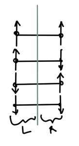
An example of a partitioned system with four total states (two spin 1/2 particles) is sketched in fig. 1.
An example of a partitioned system with eight total states (three spin 1/2 particles) is sketched in fig. 2.
The density matrix
\begin{equation}\label{eqn:qmLecture3:20}
\hat{\rho} = \ket{\Psi}\bra{\Psi}
\end{equation}
is clearly an operator as can be seen by applying it to a state
\begin{equation}\label{eqn:qmLecture3:40}
\hat{\rho} \ket{\phi} = \ket{\Psi} \lr{ \braket{ \Psi }{\phi} }.
\end{equation}
The quantity in braces is just a complex number.
After expanding the pure state \( \ket{\Psi} \) in terms of basis states for each of the two partitions
\begin{equation}\label{eqn:qmLecture3:60}
\ket{\Psi}
= \sum_{m,n} C_{m, n} \ket{m}_{\textrm{L}} \ket{n}_{\textrm{R}},
\end{equation}
With \( \textrm{L} \) and \( \textrm{R} \) implied for \( \ket{m}, \ket{n} \) indexed states respectively, this can be written
\begin{equation}\label{eqn:qmLecture3:460}
\ket{\Psi}
= \sum_{m,n} C_{m, n} \ket{m} \ket{n}.
\end{equation}
The density operator is
\begin{equation}\label{eqn:qmLecture3:80}
\hat{\rho} =
\sum_{m,n}
C_{m, n}
C_{m’, n’}^\conj
\ket{m} \ket{n}
\sum_{m’,n’}
\bra{m’} \bra{n’}.
\end{equation}
Suppose we trace over the right partition of the state space, defining such a trace as the reduced density operator \( \hat{\rho}_{\textrm{red}} \)
\begin{equation}\label{eqn:qmLecture3:100}
\begin{aligned}
\hat{\rho}_{\textrm{red}}
&\equiv
\textrm{Tr}_{\textrm{R}}(\hat{\rho}) \\
&= \sum_{\tilde{n}} \bra{\tilde{n}} \hat{\rho} \ket{ \tilde{n}} \\
&= \sum_{\tilde{n}}
\bra{\tilde{n} }
\lr{
\sum_{m,n}
C_{m, n}
\ket{m} \ket{n}
}
\lr{
\sum_{m’,n’}
C_{m’, n’}^\conj
\bra{m’} \bra{n’}
}
\ket{ \tilde{n} } \\
&=
\sum_{\tilde{n}}
\sum_{m,n}
\sum_{m’,n’}
C_{m, n}
C_{m’, n’}^\conj
\ket{m} \delta_{\tilde{n} n}
\bra{m’ }
\delta_{ \tilde{n} n’ } \\
&=
\sum_{\tilde{n}, m, m’}
C_{m, \tilde{n}}
C_{m’, \tilde{n}}^\conj
\ket{m} \bra{m’ }
\end{aligned}
\end{equation}
Computing the matrix element of \( \hat{\rho}_{\textrm{red}} \), we have
\begin{equation}\label{eqn:qmLecture3:120}
\begin{aligned}
\bra{\tilde{m}} \hat{\rho}_{\textrm{red}} \ket{\tilde{m}}
&=
\sum_{m, m’, \tilde{n}} C_{m, \tilde{n}} C_{m’, \tilde{n}}^\conj \braket{ \tilde{m}}{m} \braket{m’}{\tilde{m}} \\
&=
\sum_{\tilde{n}} \Abs{C_{\tilde{m}, \tilde{n}} }^2.
\end{aligned}
\end{equation}
This is the probability that the left partition is in state \( \tilde{m} \).
Average of an observable
Suppose we have two spin half particles. For such a system the total magnetization is
\begin{equation}\label{eqn:qmLecture3:140}
S_{\textrm{Total}} =
S_1^z
+
S_1^z,
\end{equation}
as sketched in fig. 3.
The average of some observable is
\begin{equation}\label{eqn:qmLecture3:160}
\expectation{\hatA}
= \sum_{m, n, m’, n’} C_{m, n}^\conj C_{m’, n’}
\bra{m}\bra{n} \hatA \ket{n’} \ket{m’}.
\end{equation}
Consider the trace of the density operator observable product
\begin{equation}\label{eqn:qmLecture3:180}
\textrm{Tr}( \hat{\rho} \hatA )
= \sum_{m, n} \braket{m n}{\Psi} \bra{\Psi} \hatA \ket{m, n}.
\end{equation}
Let
\begin{equation}\label{eqn:qmLecture3:200}
\ket{\Psi} = \sum_{m, n} C_{m n} \ket{m, n},
\end{equation}
so that
\begin{equation}\label{eqn:qmLecture3:220}
\begin{aligned}
\textrm{Tr}( \hat{\rho} \hatA )
&= \sum_{m, n, m’, n’, m”, n”} C_{m’, n’} C_{m”, n”}^\conj
\braket{m n}{m’, n’} \bra{m”, n”} \hatA \ket{m, n} \\
&= \sum_{m, n, m”, n”} C_{m, n} C_{m”, n”}^\conj
\bra{m”, n”} \hatA \ket{m, n}.
\end{aligned}
\end{equation}
This is just
\begin{equation}\label{eqn:qmLecture3:240}
\boxed{
\bra{\Psi} \hatA \ket{\Psi} = \textrm{Tr}( \hat{\rho} \hatA ).
}
\end{equation}
Left observables
Consider
\begin{equation}\label{eqn:qmLecture3:260}
\begin{aligned}
\bra{\Psi} \hatA_{\textrm{L}} \ket{\Psi}
&= \textrm{Tr}(\hat{\rho} \hatA_{\textrm{L}}) \\
&=
\textrm{Tr}_{\textrm{L}}
\textrm{Tr}_{\textrm{R}}
(\hat{\rho} \hatA_{\textrm{L}}) \\
&=
\textrm{Tr}_{\textrm{L}}
\lr{
\lr{
\textrm{Tr}_{\textrm{R}} \hat{\rho}
}
\hatA_{\textrm{L}})
} \\
&=
\textrm{Tr}_{\textrm{L}}
\lr{
\hat{\rho}_{\textrm{red}}
\hatA_{\textrm{L}})
}.
\end{aligned}
\end{equation}
We see
\begin{equation}\label{eqn:qmLecture3:280}
\bra{\Psi} \hatA_{\textrm{L}} \ket{\Psi}
=
\textrm{Tr}_{\textrm{L}} \lr{ \hat{\rho}_{\textrm{red}, \textrm{L}} \hatA_{\textrm{L}} }.
\end{equation}
We find that we don’t need to know the state of the complete system to answer questions about portions of the system, but instead just need \( \hat{\rho} \), a “probability operator” that provides all the required information about the partitioning of the system.
Pure states vs. mixed states
For pure states we can assign a state vector and talk about reduced scenarios. For mixed states we must work with reduced density matrix.
Example: Two particle spin half pure states
Consider
\begin{equation}\label{eqn:qmLecture3:300}
\ket{\psi_1} = \inv{\sqrt{2}} \lr{ \ket{ \uparrow \downarrow } – \ket{ \downarrow \uparrow } }
\end{equation}
\begin{equation}\label{eqn:qmLecture3:320}
\ket{\psi_2} = \inv{\sqrt{2}} \lr{ \ket{ \uparrow \downarrow } + \ket{ \uparrow \uparrow } }.
\end{equation}
For the first pure state the density operator is
\begin{equation}\label{eqn:qmLecture3:360}
\hat{\rho} = \inv{2}
\lr{ \ket{ \uparrow \downarrow } – \ket{ \downarrow \uparrow } }
\lr{ \bra{ \uparrow \downarrow } – \bra{ \downarrow \uparrow } }
\end{equation}
What are the reduced density matrices?
\begin{equation}\label{eqn:qmLecture3:340}
\begin{aligned}
\hat{\rho}_{\textrm{L}}
&= \textrm{Tr}_{\textrm{R}} \lr{ \hat{\rho} } \\
&=
\inv{2} (-1)(-1) \ket{\downarrow}\bra{\downarrow}
+\inv{2} (+1)(+1) \ket{\uparrow}\bra{\uparrow},
\end{aligned}
\end{equation}
so the matrix representation of this reduced density operator is
\begin{equation}\label{eqn:qmLecture3:380}
\hat{\rho}_{\textrm{L}}
=
\inv{2}
\begin{bmatrix}
1 & 0 \\
0 & 1
\end{bmatrix}.
\end{equation}
For the second pure state the density operator is
\begin{equation}\label{eqn:qmLecture3:400}
\hat{\rho} = \inv{2}
\lr{ \ket{ \uparrow \downarrow } + \ket{ \uparrow \uparrow } }
\lr{ \bra{ \uparrow \downarrow } + \bra{ \uparrow \uparrow } }.
\end{equation}
This has a reduced density matrice
\begin{equation}\label{eqn:qmLecture3:420}
\begin{aligned}
\hat{\rho}_{\textrm{L}}
&= \textrm{Tr}_{\textrm{R}} \lr{ \hat{\rho} } \\
&=
\inv{2} \ket{\uparrow}\bra{\uparrow}
+\inv{2} \ket{\uparrow}\bra{\uparrow} \\
&=
\ket{\uparrow}\bra{\uparrow} .
\end{aligned}
\end{equation}
This has a matrix representation
\begin{equation}\label{eqn:qmLecture3:440}
\hat{\rho}_{\textrm{L}}
=
\begin{bmatrix}
1 & 0 \\
0 & 0
\end{bmatrix}.
\end{equation}
In this second example, we have more information about the left partition. That will be seen as a zero entanglement entropy in the problem set. In contrast we have less information about the first state, and will find a non-zero positive entanglement entropy in that case.
References
[1] Jun John Sakurai and Jim J Napolitano. Modern quantum mechanics. Pearson Higher Ed, 2014.


