math and physics play

PHY2403 (QFT I). Pondering the ground state bra formula.

November 5, 2018 phy2403 , ,

[Click here for a PDF of this post with nicer formatting]

In lecture 14 we found

\begin{equation}\label{eqn:qftLecture15:60}
\ket{\Omega}
=
\evalbar{
\frac{ U(t_0, -T) \ket{0} }
{
e^{-i E_0(T – t_0)} \braket{\Omega}{0}
}
}{T \rightarrow \infty(1 – i \epsilon)},
\end{equation}
and it was stated that we can also show that
\begin{equation}\label{eqn:qftLecture15:80}
\bra{\Omega}
=
\evalbar{
\frac{ \bra{0} U(T, t_0) }
{
e^{-i E_0(T – t_0)} \braket{0}{\Omega}
}
}{T \rightarrow \infty(1 – i \epsilon)}.
\end{equation}

This second statement is actually not obvious since
\begin{equation}\label{eqn:braOmega:100}
\lr{
\frac{ U(t_0, -T) \ket{0} }
{
e^{-i E_0(T – t_0)} \braket{\Omega}{0}
}
}^\dagger
=
\frac{ \bra{0} U(-T, t_0) \ket{0} }
{
e^{+i E_0(T – t_0)} \braket{0}{\Omega}
}
\end{equation}

My first thought was that I’d written down \ref{eqn:qftLecture15:80} in my notes wrong, but this is actually also consistent with [1], which our Prof is following loosely (i.e. he is explicitly filling in many of the holes in that dense little 800 page book).

The resolution of this inconsistency is that the limit point \( \infty(1 – i \epsilon) \) doesn’t work if you just conjugate, and you’d also have to conjugate that limit, so while
\ref{eqn:braOmega:100} is correct, it is only part of the story, and should really be stated as
\begin{equation}\label{eqn:braOmega:120}
\bra{\Omega}
=
\evalbar{
\frac{ \bra{0} U(-T, t_0) \ket{0} }
{
e^{+i E_0(T – t_0)} \braket{0}{\Omega}
}
}{T \rightarrow \infty(1 + i \epsilon)}.
\end{equation}
This is awkward because now our expressions for \( \bra{\Omega} \) and \( \ket{\Omega} \) approach \( T \) from different directions, and we want to evaluate both with a single limiting argument.

To resolve this, we really have to start back with the identity expansion we used in lecture 14
\begin{equation}\label{eqn:braOmega:140}
\begin{aligned}
\bra{0} e^{-i H T}
&=
\lr{
\braket{0}{\Omega}\bra{\Omega}
+ {\int\kern-1em\sum}_n \braket{0}{n} \bra{n}
}
e^{-i H T} \\
&=
\braket{0}{\Omega}\bra{\Omega}
e^{-i E_0 T}
+ {\int\kern-1em\sum}_n \braket{0}{n} \bra{n} e^{-i E_n T}.
\end{aligned}
\end{equation}
We argued (as does the text) that approaching to as \( T( 1 – i \epsilon) \) kills off the energetic states since
\begin{equation}\label{eqn:braOmega:160}
\bra{n} e^{-i E_n T}
\rightarrow
\bra{n} e^{-i E_n T} e^{-E_n T \epsilon}
\end{equation}
and the exponential damping factor is smaller for each \( E_n > E_0 \), so it can be neglected in the large \( T \) limit, leaving
\begin{equation}\label{eqn:braOmega:180}
\bra{0} e^{-i H T}
=
\lim_{T \rightarrow \infty(1 – i \epsilon)}
\braket{0}{\Omega}\bra{\Omega}.
\end{equation}
As we did for \( \ket{\Omega} \) we can shift the large time \( T \) by a small constant (this time \( -t_0 \) instead of \( t_0 \)), to give
\begin{equation}\label{eqn:braOmega:200}
\begin{aligned}
\bra{\Omega}
&=
\lim_{T \rightarrow \infty(1 – i \epsilon)}
\frac{ \bra{0} e^{-i H T} }
{
\braket{0}{\Omega} e^{-i E_0 T}
} \\
&\approx
\lim_{T \rightarrow \infty(1 – i \epsilon)}
\frac{ \bra{0} e^{-i H (T – t_0)} }
{
\braket{0}{\Omega} e^{-i E_0 (T – t_0)}
} \\
&=
\lim_{T \rightarrow \infty(1 – i \epsilon)}
\frac{ \bra{0} e^{i H_0( T – t_0)} e^{-i H (T – t_0)} }
{
\braket{0}{\Omega} e^{-i E_0 (T – t_0)}
} \\
&=
\lim_{T \rightarrow \infty(1 – i \epsilon)}
\frac{ \bra{0} U(T, t_0) }
{
\braket{0}{\Omega} e^{-i E_0 (T – t_0)}
},
\end{aligned}
\end{equation}
where the projective property \( \bra{0} e^{i H_0 \alpha} = \bra{0} \) has been used to insert a no-op (i.e. \( \bra{0} H_0 = 0 \)). This recovers the result stated in class (also: eq. (4.29) in the text.)

References

[1] Michael E Peskin and Daniel V Schroeder. An introduction to Quantum Field Theory. Westview, 1995.

Analysis of incorrect problem solution attempt (non-relativistic QFT massive scalar field with quadratic interaction)

November 1, 2018 phy2403 , ,

[Click here for a PDF of this post with nicer formatting]

An incorrect start at a field theory problem.

The following is a problem from the second PHY2403 problem set, and the start of a solution attempt I made. I’m not posting this because it shows how to do the problem, but because it was a useful problem to show that I didn’t understand a lot of the problem statement.
Understanding where I went wrong is actually pretty useful in this case.

Problem: Playing with the non-relativistic limit

Consider a real scalar relativistic field theory of mass m with \( \lambda \phi^4 \) interaction. Let there be \( N \) particles of momenta labeled by \( p_1,\cdots, p_N\), whose energies are such that they are insufficient to create any new particles. Nevertheless, the particles can scatter and exchange momenta. In what follows you will study this N-particle nonrelativistic limit in some detail.

  1. Write down the Hamiltonian of the field theory, including the interaction term, restricted to the N-particle sector of Hilbert space. (Use the creation and annihilation operator representation, i.e. write the result as sums of products of creation and annihilation operators of particles of various momenta.)
  2. Does the resulting Hamiltonian preserve particle number? Is there an associated symmetry? What is the operator that generates it?
  3. Consider now the interaction term in your reduced (to the N-particle sector of Hilbert space) Hamiltonian. How does a typical interaction term (for given configurations of momenta) act on an N-particle state? What kinds of scattering processes does it describe?
  4. What do you think is the potential, in x-space, that allows the various particles to scatter and exchange momentum? How would you describe the resulting nonrelativistic quantum system to friends who never took QFT but are well-versed in quantum mechanics?

Incorrect answer attempt.

The Lagrangian density of a massive scalar field with a \( \lambda \phi^4 \) interaction has the form
\begin{equation}\label{eqn:Nparticle:20}
\LL = \inv{2} \partial_\mu \phi \partial^\mu \phi – \inv{2} m^2 \phi^2 – \lambda \phi^4.
\end{equation}
The corresponding Hamiltonian is
\begin{equation}\label{eqn:Nparticle:40}
H = \inv{2} \int d^3x \lr{ \pi^2 + \frac{m^2}{2} (\spacegrad \phi)^2 + m^2 \phi^2 } + \lambda \int d^3 x \phi^4.
\end{equation}
In terms of creation and annihilation operators, we know the form of the non-interaction portion of the Hamiltonian, which in normal order is
\begin{equation}\label{eqn:Nparticle:60}
H_0 = \int \frac{d^3 p}{(2 \pi)^3} \omega_\Bp a_\Bp^\dagger a_\Bp,
\end{equation}
but the interaction contribution is much messier
\begin{equation}\label{eqn:Nparticle:80}
\begin{aligned}
H_{\text{int}}
&=
\lambda \int d^3 x \frac{ d^3 p d^3 k d^3 q d^3 s}{4 (2 \pi)^{12} \sqrt{
\omega_\Bp \omega_\Bk \omega_\Bq \omega_\Bs
} }
\lr{ a_\Bp e^{-i p \cdot x} + a_\Bp e^{i p \cdot x} }
\lr{ a_\Bk e^{-i k \cdot x} + a_\Bk e^{i k \cdot x} }
\lr{ a_\Bq e^{-i q \cdot x} + a_\Bq e^{i q \cdot x} }
\lr{ a_\Bs e^{-i s \cdot x} + a_\Bs e^{i s \cdot x} } \\
&=
\lambda \int d^3 x \frac{ d^3 p d^3 k d^3 q d^3 s}{4 (2 \pi)^{12} \sqrt{
\omega_\Bp \omega_\Bk \omega_\Bq \omega_\Bs
} }
\lr{ a_\Bp e^{-i \omega_\Bp t + i \Bp \cdot \Bx} + a_\Bp e^{i \omega_\Bp t – i \Bp \cdot \Bx} }
\lr{ a_\Bk e^{-i \omega_\Bk t + i \Bk \cdot \Bx} + a_\Bk e^{i \omega_\Bk t – i \Bk \cdot \Bx} } \\
&\quad \lr{ a_\Bq e^{-i \omega_\Bq t + i \Bq \cdot \Bx} + a_\Bq e^{i \omega_\Bq t – i \Bq \cdot \Bx} }
\lr{ a_\Bs e^{-i \omega_\Bs t + i \Bs \cdot \Bx} + a_\Bs e^{i \omega_\Bs t – i \Bs \cdot \Bx} } \\
&=
\lambda \int \frac{ d^3 p d^3 k d^3 q d^3 s}{4 (2 \pi)^{9} \sqrt{
\omega_\Bp \omega_\Bk \omega_\Bq \omega_\Bs
} }
\Big(
a_\Bp a_\Bk a_\Bq a_\Bs e^{-i (\omega_\Bp + \omega_\Bk + \omega_\Bq + \omega_\Bs)t} \delta^3( \Bp + \Bk + \Bq + \Bs ) \\
&\qquad +
a_\Bp a_\Bk a_\Bq a_\Bs^\dagger e^{-i (\omega_\Bp + \omega_\Bk + \omega_\Bq – \omega_\Bs)t} \delta^3( \Bp + \Bk + \Bq – \Bs ) \\
&\qquad \\
&\qquad + \cdots \\
&\qquad +
a_\Bp^\dagger a_\Bk^\dagger a_\Bq^\dagger a_\Bs^\dagger e^{-i (-\omega_\Bp – \omega_\Bk – \omega_\Bq – \omega_\Bs)t} \delta^3( -\Bp – \Bk – \Bq – \Bs )
\Big) \\
&=
\lambda \int \frac{ d^3 p d^3 k d^3 q }{4 (2 \pi)^{9}
}
\Big(
\inv{\sqrt{
\omega_\Bp \omega_\Bk \omega_\Bq \omega_{-\Bp – \Bk – \Bq}
}}
a_\Bp a_\Bk a_\Bq a_{-\Bp -\Bk – \Bq} e^{-i (\omega_\Bp + \omega_\Bk + \omega_\Bq + \omega_{-\Bp -\Bk -\Bq})t} \\
&\qquad +
\inv{\sqrt{
\omega_\Bp \omega_\Bk \omega_\Bq \omega_{\Bp + \Bk + \Bq}
}}
a_\Bp a_\Bk a_\Bq a_{\Bp + \Bk + \Bq}^\dagger e^{-i (\omega_\Bp + \omega_\Bk + \omega_\Bq – \omega_{\Bp + \Bk + \Bq})t} \\
&\qquad +
\cdots \\
&\qquad +
\inv{\sqrt{
\omega_\Bp \omega_\Bk \omega_\Bq \omega_{-\Bp – \Bk – \Bq}
}}
a_\Bp^\dagger a_\Bk^\dagger a_\Bq^\dagger a_{-\Bp -\Bk -\Bq}^\dagger e^{-i (-\omega_\Bp – \omega_\Bk – \omega_\Bq – \omega_{-\Bp -\Bk -\Bq})t}
\Big)
\end{aligned}
\end{equation}
Assuming we can normal order these terms as in \( H_0 \), we can rewrite the interaction as
\begin{equation}\label{eqn:Nparticle:100}
\begin{aligned}
H_{\text{int}}
&=
\lambda \int \frac{ d^3 p d^3 k d^3 q }{4 (2 \pi)^{9} }
\Big(
\binom{4}{0}
\inv{\sqrt{
\omega_\Bp \omega_\Bk \omega_\Bq \omega_{-\Bp – \Bk – \Bq}
}}
a_\Bp a_\Bk a_\Bq a_{-\Bp -\Bk – \Bq} e^{-i (\omega_\Bp + \omega_\Bk + \omega_\Bq + \omega_{-\Bp -\Bk -\Bq})t} \\
&\qquad +
\binom{4}{1}
\inv{\sqrt{
\omega_\Bp \omega_\Bk \omega_\Bq \omega_{\Bp – \Bk – \Bq}
}}
a_\Bp^\dagger a_\Bk a_\Bq a_{\Bp – \Bk – \Bq} e^{-i (-\omega_\Bp + \omega_\Bk + \omega_\Bq + \omega_{\Bp – \Bk – \Bq})t} \\
&\qquad +
\binom{4}{2}
\inv{\sqrt{
\omega_\Bp \omega_\Bk \omega_\Bq \omega_{\Bp + \Bk – \Bq}
}}
a_\Bp^\dagger a_\Bk^\dagger a_\Bq a_{\Bp + \Bk – \Bq} e^{-i (-\omega_\Bp – \omega_\Bk + \omega_\Bq + \omega_{\Bp + \Bk – \Bq})t} \\
&\qquad +
\binom{4}{3}
\inv{\sqrt{
\omega_\Bp \omega_\Bk \omega_\Bq \omega_{\Bp + \Bk _ \Bq}
}}
a_\Bp^\dagger a_\Bk^\dagger a_\Bq^\dagger a_{\Bp + \Bk + \Bq} e^{-i (-\omega_\Bp – \omega_\Bk – \omega_\Bq + \omega_{\Bp + \Bk + \Bq})t} \\
&\qquad +
\binom{4}{4}
\inv{\sqrt{
\omega_\Bp \omega_\Bk \omega_\Bq \omega_{-\Bp – \Bk – \Bq}
}}
a_\Bp^\dagger a_\Bk^\dagger a_\Bq^\dagger a_{-\Bp -\Bk -\Bq}^\dagger e^{-i (-\omega_\Bp – \omega_\Bk – \omega_\Bq – \omega_{-\Bp -\Bk -\Bq})t}
\Big)
\end{aligned}
\end{equation}

If we restrict the allowed momenta to the discrete set \( \Bp \in \setlr{ \Bp_1, \Bp_2, \cdots \Bp_N} \), the total Hamiltonian including the interaction term
takes the form
\begin{equation}\label{eqn:Nparticle:120}
\begin{aligned}
\text{\(:H:\)} &=
\sum_{i = 1}^N \omega_{\Bp_i} a_{\Bp_i}^\dagger a_{\Bp_i}
+
\frac{
\lambda
}{4 }
\sum_{j,m,n = 1}^N
\Big(
\binom{4}{0}
\inv{\sqrt{
\omega_{\Bp_j} \omega_{\Bp_m} \omega_{\Bp_n} \omega_{-{\Bp_j} – {\Bp_m} – {\Bp_n}}
}}
a_{\Bp_j} a_{\Bp_m} a_{\Bp_n} a_{-\Bp -\Bk – \Bq} e^{-i (\omega_{\Bp_j} + \omega_{\Bp_m} + \omega_{\Bp_n} + \omega_{-{\Bp_j} -{\Bp_m} -{\Bp_n}})t} \\
&\qquad +
\binom{4}{1}
\inv{\sqrt{
\omega_{\Bp_j} \omega_{\Bp_m} \omega_{\Bp_n} \omega_{{\Bp_j} – {\Bp_m} – {\Bp_n}}
}}
a_{\Bp_j}^\dagger a_{\Bp_m} a_{\Bp_n} a_{{\Bp_j} – {\Bp_m} – {\Bp_n}} e^{-i (-\omega_{\Bp_j} + \omega_{\Bp_m} + \omega_{\Bp_n} + \omega_{{\Bp_j} – {\Bp_m} – {\Bp_n}})t} \\
&\qquad +
\binom{4}{2}
\inv{\sqrt{
\omega_{\Bp_j} \omega_{\Bp_m} \omega_{\Bp_n} \omega_{{\Bp_j} + {\Bp_m} – {\Bp_n}}
}}
a_{\Bp_j}^\dagger a_{\Bp_m}^\dagger a_{\Bp_n} a_{{\Bp_j} + {\Bp_m} – {\Bp_n}} e^{-i (-\omega_{\Bp_j} – \omega_{\Bp_m} + \omega_{\Bp_n} + \omega_{{\Bp_j} + {\Bp_m} – {\Bp_n}})t} \\
&\qquad +
\binom{4}{3}
\inv{\sqrt{
\omega_{\Bp_j} \omega_{\Bp_m} \omega_{\Bp_n} \omega_{{\Bp_j} + {\Bp_m} – {\Bp_n}}
}}
a_{\Bp_j}^\dagger a_{\Bp_m}^\dagger a_{\Bp_n}^\dagger a_{{\Bp_j} + {\Bp_m} + {\Bp_n}} e^{-i (-\omega_{\Bp_j} – \omega_{\Bp_m} – \omega_{\Bp_n} + \omega_{{\Bp_j} + {\Bp_m} + {\Bp_n}})t} \\
&\qquad +
\binom{4}{4}
\inv{\sqrt{
\omega_{\Bp_j} \omega_{\Bp_m} \omega_{\Bp_n} \omega_{-{\Bp_j} – {\Bp_m} – {\Bp_n}}
}}
a_{\Bp_j}^\dagger a_{\Bp_m}^\dagger a_{\Bp_n}^\dagger a_{-{\Bp_j} -{\Bp_m} -{\Bp_n}}^\dagger e^{-i (-\omega_{\Bp_j} – \omega_{\Bp_m} – \omega_{\Bp_n} – \omega_{-{\Bp_j} -{\Bp_m} -{\Bp_n}})t}
\Big)
\end{aligned}
\end{equation}

When we did the same sort of calculation for \( (\spacegrad \phi)^2 + m^2 \phi^2 \) all the time dependent terms cancelled nicely, but that isn’t obviously the case here.
However, we haven’t used the non-relativistic (low energy) constraint. That constraint can be expressed as \( \Bp^2 \ll m^2 \), in which case \( \omega_\Bp = \sqrt{ \Bp^2 + m^2 } \sim m \), the mass of each of the particles. Incorporating that into our N-particle Hamiltonian, we have
\begin{equation}\label{eqn:Nparticle:140}
\begin{aligned}
\text{\(:H:\)} &=
\sum_{i = 1}^N \omega_{\Bp_i} a_{\Bp_i}^\dagger a_{\Bp_i}
+
\frac{
\lambda
}{4 m^2 }
\sum_{j,m,n = 1}^N
\Big(
\binom{4}{0}
a_{\Bp_j} a_{\Bp_m} a_{\Bp_n} a_{-\Bp -\Bk – \Bq} e^{- 4 i m t} \\
&\qquad +
\binom{4}{1}
a_{\Bp_j}^\dagger a_{\Bp_m} a_{\Bp_n} a_{{\Bp_j} – {\Bp_m} – {\Bp_n}} e^{-3 i m t} \\
&\qquad +
\binom{4}{2}
a_{\Bp_j}^\dagger a_{\Bp_m}^\dagger a_{\Bp_n} a_{{\Bp_j} + {\Bp_m} – {\Bp_n}} \\
&\qquad +
\binom{4}{3}
a_{\Bp_j}^\dagger a_{\Bp_m}^\dagger a_{\Bp_n}^\dagger a_{{\Bp_j} + {\Bp_m} + {\Bp_n}} e^{ 3 i m t } \\
&\qquad +
\binom{4}{4}
a_{\Bp_j}^\dagger a_{\Bp_m}^\dagger a_{\Bp_n}^\dagger a_{-{\Bp_j} -{\Bp_m} -{\Bp_n}}^\dagger e^{4 i m t}
\Big).
\end{aligned}
\end{equation}

The only annoying aspect to this Hamiltonian is the \( a_{{\Bp_j} + {\Bp_m} – {\Bp_n}} \) operator in the interaction term, which is not clear to me how to interpret. That seems to imply that it is possible to create particles with linear combinations of momentum that may not be in the original set of \( N \) particle momenta. I think that this can be further fudged by invoking the non-relativistic constraint again, and decreeing that each of the uniquely indexed creation and annihilation operators are distinguishable only by index, so we can write the N-particle non-relativistic sector Hamiltonian as
\begin{equation}\label{eqn:Nparticle:170}
\text{\(:H:\)} =
\sum_{i = 1}^N \omega_{\Bp_i}
a_{i}^\dagger a_{i}
+
\frac{
3 \lambda
}{2 m^2 }
\sum_{r,s,t,u = 1}^N
a_{r}^\dagger a_{s}^\dagger a_{t} a_{u}.
\end{equation}

Commentary.

While there are a few things that are not wrong above, those correct parts are liberally mixed with a few fundamental errors.

Even before getting to the fundamential errors, there are a few minor issues too. For example, I don’t think that there is anything strictly wrong with the expansion of \ref{eqn:Nparticle:100} for example, although it appears that I confused myself by actually evaluating the delta function instead of just identifying it, something like:
\begin{equation}\label{eqn:Nparticle:190}
\begin{aligned}
H_{\text{int}}
&=
\frac{\lambda}{4} \int \frac{ d^3 p d^3 k d^3 q d^3 s}{(2 \pi)^{12} \sqrt{ \omega_\Bp \omega_\Bk \omega_\Bq \omega_\Bs } }
\Big(
\binom{4}{0}
\delta^3( \Bp + \Bk + \Bq + \Bs )
a_\Bp a_\Bk a_\Bq a_\Bs e^{-i (\omega_\Bp + \omega_\Bk + \omega_\Bq + \omega_\Bs) t} \\
&\qquad +
\binom{4}{1}
\delta^3( -\Bp + \Bk + \Bq + \Bs )
a_\Bp^\dagger a_\Bk a_\Bq a_\Bs e^{-i (-\omega_\Bp + \omega_\Bk + \omega_\Bq + \omega_\Bs)t} \\
&\qquad +
\binom{4}{2}
\delta^3( -\Bp – \Bk + \Bq + \Bs )
a_\Bp^\dagger a_\Bk^\dagger a_\Bq a_\Bs e^{-i (-\omega_\Bp – \omega_\Bk + \omega_\Bq + \omega_\Bs)t} \\
&\qquad +
\binom{4}{3}
\delta^3( -\Bp – \Bk – \Bq + \Bs )
a_\Bp^\dagger a_\Bk^\dagger a_\Bq^\dagger a_\Bs e^{-i (-\omega_\Bp – \omega_\Bk – \omega_\Bq + \omega_\Bs)t} \\
&\qquad +
\binom{4}{4}
\delta^3( -\Bp – \Bk – \Bq – \Bs )
a_\Bp^\dagger a_\Bk^\dagger a_\Bq^\dagger a_\Bs^\dagger e^{-i (-\omega_\Bp – \omega_\Bk – \omega_\Bq – \omega_\Bs)t}
\Big)
\end{aligned}
\end{equation}

So much of QFT is expressed in terms of delta functions, yet I tend to view them as something to be eliminated instead of retained. One lesson is that delta functions in QFT should be embraced, and had I done so in this case, I would have had a better chance of understanding the scattering part of the question that came later. One role of the delta function actually appears to be critical to the scattering question, as it actually encodes the constraints that lead to conservation of momentum in a “scattering process” related to the interaction term of the Hamiltonian.

I didn’t understand what was meant by a scattering process, but that was related to another more fundamental misunderstanding. That screw up was in my interpretation of what was meant by the “N particle sector of the Hilbert space.” In my reading of that phrase I tossed out “Hilbert space” as irrelevant. Part of that was somewhat reactionary, as it seems to me that Hilbert space is tossed around in so much QM in a way that makes it seem more rigorous, but we never touch on the scary mathematics that rigorously defines what a Hilbert space is. It seems to me that the phrase “Hilbert space” is often used as a pretentious way of saying “complex inner product space”. It has a more precise meaning to Mathematicians, but I don’t think that most physicists understand that meaning (and most certainly most students of QM don’t).

So, long story short, I interpreted “N particle sector of the Hilbert space” as “N particle sector” and though that meant I had to somehow discretize the system, introducing N discrete momenta into the mix. Here’s an example, using the non-interaction Hamiltonian, of exactly how I did that:
\begin{equation}\label{eqn:Nparticle:210}
\int \frac{d^3 p}{(2 \pi)^3} \omega_\Bp a_\Bp^\dagger a_\Bp \rightarrow \sum_{i = 1}^N \omega_\Bp a_\Bp^\dagger a_\Bp.
\end{equation}

This is wrong! I actually clued into part of the trouble with this, but didn’t know what the root cause was. I fudged around that my dropping the problematic side effects of having evaluated the delta function, which lead me to have terms like \( a_{\Bp + \Bq – \Bk} \) in the expansion of the interaction Hamiltonian. I couldn’t see how creation and annihilation operators that are associated with arbitrary linear combinations of the other momenta could maintain an \( N \) particle system. Those linear combinations could easily lie outside of the set of the original \( N \) particle system that I constructed in my discretization.

In office hours, Professor Poppitz had me work a small problem to illustrate the error in my ways, specifically applying the Hamiltonian to a two momentum state
\begin{equation}\label{eqn:Nparticle:230}
\begin{aligned}
H \ket{\Bp_1 \Bp_2}
&=
\lr{
\int \frac{d^3}{(2 \pi)^3}
a_\Bp^\dagger
a_\Bp
}
a_{\Bp_1}^\dagger
a_{\Bp_2}^\dagger
\ket{0} \\
&=
\int \frac{d^3}{(2 \pi)^3} \omega_\Bp
a_\Bp^\dagger
\lr{
a_{\Bp_1}^\dagger a_\Bp
+ (2 \pi) \delta^3(\Bp -\Bp_1)
}
a_{\Bp_2}^\dagger
\ket{0} \\
&=
\int \frac{d^3}{(2 \pi)^3} \omega_\Bp
a_\Bp^\dagger
a_{\Bp_1}^\dagger a_\Bp
a_{\Bp_2}^\dagger
\ket{0}
+
\omega_{\Bp_1}
a_{\Bp_1}^\dagger
a_{\Bp_2}^\dagger
\ket{0} \\
&=
\int \frac{d^3}{(2 \pi)^3} \omega_\Bp
a_\Bp^\dagger
a_{\Bp_1}^\dagger
\lr{
a_{\Bp_2}^\dagger
a_\Bp
+ (2 \pi)^3 \delta^3(\Bp – \Bp_2)
}
\ket{0}
+
\omega_{\Bp_1}\ket{\Bp_1 \Bp_2} \\
&=
\lr{ \omega_{\Bp_1} + \omega_{\Bp_2} }
\ket{\Bp_1 \Bp_2}.
\end{aligned}
\end{equation}
Observe that the Hamiltonian operates on a two momentum state, returning that state scaled by the energy associated with the sum of the momenta. Given an two particle subspace of all the possible two momentum states, perhaps with a basis like \( \setlr{\ket{\Bp_1 \Bp_2}, \ket{\Bp_3 \Bp_4}, \cdots } \), the Hamiltonian provides a mapping from that set onto itself, as it scales the states in question, but does not convert two particle states into combinations of one and three momentum states (say). This is not the case with the interaction Hamiltonian, as an operation like \( \int a^\dagger a^\dagger a^\dagger a \) doesn’t preserve a two momentum state. Example
\begin{equation}\label{eqn:Nparticle:250}
\begin{aligned}
\int
&\frac{d^3 p}{(2\pi)^3\sqrt{ 2\omega_\Bp}}
\frac{d^3 q}{(2\pi)^3\sqrt{ 2\omega_\Bq}}
\frac{d^3 r}{(2\pi)^3\sqrt{ 2\omega_\Br}}
\frac{d^3 s}{(2\pi)^3\sqrt{ 2\omega_\Bs}}
\delta^3(\Bp + \Bq + \Br -\Bs)
a_\Bp^\dagger
a_\Bq^\dagger
a_\Br^\dagger
a_\Bs
\ket{ \Bp_1 \Bp_2 } \\
&=
\int
\frac{d^3 p}{(2\pi)^3\sqrt{ 2\omega_\Bp}}
\frac{d^3 q}{(2\pi)^3\sqrt{ 2\omega_\Bq}}
\frac{d^3 r}{(2\pi)^3\sqrt{ 2\omega_\Br}}
\frac{d^3 s}{(2\pi)^3\sqrt{ 2\omega_\Bs}}
\delta^3(\Bp + \Bq + \Br -\Bs)
a_\Bp^\dagger
a_\Bq^\dagger
a_\Br^\dagger
a_\Bs
a_{\Bp_1}^\dagger
a_{\Bp_2}^\dagger
\ket{0} \\
&=
\int
\frac{d^3 p}{(2\pi)^3\sqrt{ 2\omega_\Bp}}
\frac{d^3 q}{(2\pi)^3\sqrt{ 2\omega_\Bq}}
\frac{d^3 r}{(2\pi)^3\sqrt{ 2\omega_\Br}}
\frac{d^3 s}{(2\pi)^3\sqrt{ 2\omega_\Bs}}
\delta^3(\Bp + \Bq + \Br -\Bs)
a_\Bp^\dagger
a_\Bq^\dagger
a_\Br^\dagger
\lr{
a_{\Bp_1}^\dagger
a_\Bs
+ (2 \pi)^3 \delta^3(\Bp_1 -\Bs)
}
a_{\Bp_2}^\dagger
\ket{0} \\
&=
\int
\frac{d^3 p}{(2\pi)^3\sqrt{ 2\omega_\Bp}}
\frac{d^3 q}{(2\pi)^3\sqrt{ 2\omega_\Bq}}
\frac{d^3 r}{(2\pi)^3\sqrt{ 2\omega_\Br}}
\frac{d^3 s}{(2\pi)^3\sqrt{ 2\omega_\Bs}}
\delta^3(\Bp + \Bq + \Br -\Bs)
a_\Bp^\dagger
a_\Bq^\dagger
a_\Br^\dagger
a_{\Bp_1}^\dagger
\lr{
a_{\Bp_2}^\dagger
a_\Bs
+ (2\pi)^3 \delta^3(\Bp_2 – \Bs)
}
\ket{0} \\
&\quad +
\int
\frac{d^3 p}{(2\pi)^3\sqrt{ 2\omega_\Bp}}
\frac{d^3 q}{(2\pi)^3\sqrt{ 2\omega_\Bq}}
\frac{d^3 r}{(2\pi)^3\sqrt{ 2\omega_\Br}}
\inv{\sqrt{ 2\omega_{\Bp_1}}}
\delta^3(\Bp + \Bq + \Br -\Bp_1)
a_\Bp^\dagger
a_\Bq^\dagger
a_\Br^\dagger
a_{\Bp_2}^\dagger
\ket{0} \\
&=
\inv{\sqrt{ 2\omega_{\Bp_2}}}
\lr{
\int
\frac{d^3 p}{(2\pi)^3\sqrt{ 2\omega_\Bp}}
\frac{d^3 q}{(2\pi)^3\sqrt{ 2\omega_\Bq}}
\frac{d^3 r}{(2\pi)^3\sqrt{ 2\omega_\Br}}
\delta^3(\Bp + \Bq + \Br -{\Bp_2})
}
\ket{\Bp \Bq \Br \Bp_1} \\
&\quad +
\inv{\sqrt{ 2\omega_{\Bp_1}}}
\lr{
\int
\frac{d^3 p}{(2\pi)^3\sqrt{ 2\omega_\Bp}}
\frac{d^3 q}{(2\pi)^3\sqrt{ 2\omega_\Bq}}
\frac{d^3 r}{(2\pi)^3\sqrt{ 2\omega_\Br}}
\delta^3(\Bp + \Bq + \Br -\Bp_1)
}
\ket{ \Bp \Bq \Br \Bp_2 }.
\end{aligned}
\end{equation}
Such a term from the interaction Hamiltonian maps a two momentum state to a four momentum state. Notice how the continuous representation is critical to this evaluation, as well as that the action of the non-interaction Hamiltonian on a two (or N) momentum state. Attempting any sort of discretization leaves you with an operator that cannot be evaluated.

Observe that only the \( (a^\dagger)^2 a^2 \) terms in the interaction will map \((1,2,3,\cdots,N)\)-momentum states to \((1,2,3,\cdots,N)\)-momentum states, so the language that I didn’t understand “N particle sector of the Hilbert” space was really an encoded instruction to retain only those interaction terms. I did exactly that because intuition told me to do so (and didn’t justify why I did so), but I had the wrong reasons for making that selection. I knew there was something wrong, but didn’t know what it was. What I should have done was go back to basics and root out all the aspects of the problem statement that I did not understand, and ask about those. If I had done so (in a timely fashion, and not at the last minute when I attempted this problem), then I wouldn’t have gone down a dead end path that lead to more confusion. I didn’t even get to the interesting part of this problem, which was to show the correspondence between the QFT picture and the classical QM picture. I’ll still attempt to do so, despite having lost my window to get credit for that work.

PHY2403H Quantum Field Theory. Lecture 14: Time evolution, Hamiltonian perturbation, ground state. Taught by Prof. Erich Poppitz

October 29, 2018 phy2403 , , , , , ,

[Click here for a PDF of this post with nicer formatting]

DISCLAIMER: Very rough notes from class, with some additional side notes.

These are notes for the UofT course PHY2403H, Quantum Field Theory, taught by Prof. Erich Poppitz, fall 2018.

Review

Given a field \( \phi(t_0, \Bx) \), satisfying the commutation relations
\begin{equation}\label{eqn:qftLecture14:20}
\antisymmetric{\pi(t_0, \Bx)}{\phi(t_0, \By)} = -i \delta(\Bx – \By)
\end{equation}
we introduced an interaction picture field given by
\begin{equation}\label{eqn:qftLecture14:40}
\phi_I(t, x) = e^{i H_0(t- t_0)} \phi(t_0, \Bx) e^{-iH_0(t – t_0)}
\end{equation}
related to the Heisenberg picture representation by
\begin{equation}\label{eqn:qftLecture14:60}
\phi_H(t, x)
= e^{i H(t- t_0)} \phi(t_0, \Bx) e^{-iH(t – t_0)}
= U^\dagger(t, t_0) \phi_I(t, \Bx) U(t, t_0),
\end{equation}
where \( U(t, t_0) \) is the time evolution operator.
\begin{equation}\label{eqn:qftLecture14:80}
U(t, t_0) =
e^{i H_0(t – t_0)}
e^{-i H(t – t_0)}
\end{equation}
We argued that
\begin{equation}\label{eqn:qftLecture14:100}
i \PD{t}{} U(t, t_0) = H_{\text{I,int}}(t) U(t, t_0)
\end{equation}
We found the glorious expression
\begin{equation}\label{eqn:qftLecture14:120}
\boxed{
\begin{aligned}
U(t, t_0)
&= T \exp{\lr{ -i \int_{t_0}^t H_{\text{I,int}}(t’) dt’}} \\
&=
\sum_{n = 0}^\infty \frac{(-i)^n}{n!} \int_{t_0}^t dt_1 dt_2 \cdots dt_n T\lr{ H_{\text{I,int}}(t_1) H_{\text{I,int}}(t_2) \cdots H_{\text{I,int}}(t_n) }
\end{aligned}
}
\end{equation}

However, what we are really after is
\begin{equation}\label{eqn:qftLecture14:140}
\bra{\Omega} T(\phi(x_1) \cdots \phi(x_n)) \ket{\Omega}
\end{equation}
Such a product has many labels and names, and we’ll describe it as “vacuum expectation values of time-ordered products of arbitrary #’s of local Heisenberg operators”.

Perturbation

Following section 4.2, [1].

\begin{equation}\label{eqn:qftLecture14:160}
\begin{aligned}
H &= \text{exact Hamiltonian} = H_0 + H_{\text{int}}
\\
H_0 &= \text{free Hamiltonian.
}
\end{aligned}
\end{equation}
We know all about \( H_0 \) and assume that it has a lowest (ground state) \( \ket{0} \), the “vacuum” state of \( H_0 \).

\( H \) has eigenstates, in particular \( H \) is assumed to have a unique ground state \( \ket{\Omega} \) satisfying
\begin{equation}\label{eqn:qftLecture14:180}
H \ket{\Omega} = \ket{\Omega} E_0,
\end{equation}
and has states \( \ket{n} \), representing excited (non-vacuum states with energies > \( E_0 \)).
These states are assumed to be a complete basis
\begin{equation}\label{eqn:qftLecture14:200}
\mathbf{1} = \ket{\Omega}\bra{\Omega} + \sum_n \ket{n}\bra{n} + \int dn \ket{n}\bra{n}.
\end{equation}
The latter terms may be written with a superimposed sum-integral notation as
\begin{equation}\label{eqn:qftLecture14:440}
\sum_n + \int dn
=
{\int\kern-1em\sum}_n,
\end{equation}
so the identity operator takes the more compact form
\begin{equation}\label{eqn:qftLecture14:460}
\mathbf{1} = \ket{\Omega}\bra{\Omega} + {\int\kern-1em\sum}_n \ket{n}\bra{n}.
\end{equation}

For some time \( T \) we have
\begin{equation}\label{eqn:qftLecture14:220}
e^{-i H T} \ket{0} = e^{-i H T}
\lr{
\ket{\Omega}\braket{\Omega}{0} + {\int\kern-1em\sum}_n \ket{n}\braket{n}{0}
}.
\end{equation}

We now wish to argue that the \( {\int\kern-1em\sum}_n \) term can be ignored.

Argument 1:

This is something of a fast one, but one can consider a formal transformation \( T \rightarrow T(1 – i \epsilon) \), where \( \epsilon \rightarrow 0^+ \), and consider very large \( T \). This gives
\begin{equation}\label{eqn:qftLecture14:240}
\begin{aligned}
\lim_{T \rightarrow \infty, \epsilon \rightarrow 0^+}
e^{-i H T(1 – i \epsilon)} \ket{0}
&=
\lim_{T \rightarrow \infty, \epsilon \rightarrow 0^+}
e^{-i H T(1 – i \epsilon)}
\lr{
\ket{\Omega}\braket{\Omega}{0} + {\int\kern-1em\sum}_n \ket{n}\braket{n}{0}
} \\
&=
\lim_{T \rightarrow \infty, \epsilon \rightarrow 0^+}
e^{-i E_0 T – E_0 \epsilon T}
\ket{\Omega}\braket{\Omega}{0} + {\int\kern-1em\sum}_n e^{-i E_n T – \epsilon E_n T} \ket{n}\braket{n}{0} \\
&=
\lim_{T \rightarrow \infty, \epsilon \rightarrow 0^+}
e^{-i E_0 T – E_0 \epsilon T}
\lr{
\ket{\Omega}\braket{\Omega}{0} + {\int\kern-1em\sum}_n e^{-i (E_n -E_0) T – \epsilon T (E_n – E_0)} \ket{n}\braket{n}{0}
}
\end{aligned}
\end{equation}
The limits are evaluated by first taking \( T \) to infinity, then only after that take \( \epsilon \rightarrow 0^+ \). Doing this, the sum is dominated by the ground state contribution, since each excited state also has a \( e^{-\epsilon T(E_n – E_0)} \) suppression factor (in addition to the leading suppression factor).

Argument 2:

With the hand waving required for the argument above, it’s worth pointing other (less formal) ways to arrive at the same result. We can write
\begin{equation}\label{eqn:qftLecture14:260}
sectionumInt \ket{n}\bra{n} \rightarrow
\sum_k \int \frac{d^3 p}{(2 \pi)^3} \ket{\Bp, k}\bra{\Bp, k}
\end{equation}
where \( k \) is some unknown quantity that we are summing over.
If we have
\begin{equation}\label{eqn:qftLecture14:280}
H \ket{\Bp, k} = E_{\Bp, k} \ket{\Bp, k},
\end{equation}
then
\begin{equation}\label{eqn:qftLecture14:300}
e^{-i H T} sectionumInt \ket{n}\bra{n}
=
\sum_k \int \frac{d^3 p}{(2 \pi)^3} \ket{\Bp, k} e^{-i E_{\Bp, k}} \bra{\Bp, k}.
\end{equation}
If we take matrix elements
\begin{equation}\label{eqn:qftLecture14:320}
\begin{aligned}
\bra{A}
e^{-i H T} sectionumInt \ket{n}\bra{n} \ket{B}
&=
\sum_k \int \frac{d^3 p}{(2 \pi)^3} \braket{A}{\Bp, k} e^{-i E_{\Bp, k}} \braket{\Bp, k}{B} \\
&=
\sum_k \int \frac{d^3 p}{(2 \pi)^3} e^{-i E_{\Bp, k}} f(\Bp).
\end{aligned}
\end{equation}
If we assume that \( f(\Bp) \) is a well behaved smooth function, we have “infinite” frequency oscillation within the envelope provided by the amplitude of that function, as depicted in fig. 1.
The Riemann-Lebesgue lemma [2] describes such integrals, the result of which is that such an integral goes to zero. This is a different sort of hand waving argument, but either way, we can argue that only the ground state contributes to the sum \ref{eqn:qftLecture14:220} above.

fig. 1. High frequency oscillations within envelope of well behaved function.


Ground state of the perturbed Hamiltonian.

With the excited states ignored, we are left with
\begin{equation}\label{eqn:qftLecture14:340}
e^{-i H T} \ket{0} = e^{-i E_0 T} \ket{\Omega}\braket{\Omega}{0}
\end{equation}
in the \( T \rightarrow \infty(1 – i \epsilon) \) limit. We can now write the ground state as

\begin{equation}\label{eqn:qftLecture14:360}
\begin{aligned}
\ket{\Omega}
&=
\evalbar{
\frac{ e^{i E_0 T – i H T } \ket{0} }{
\braket{\Omega}{0}
}
}{ T \rightarrow \infty(1 – i \epsilon) } \\
&=
\evalbar{
\frac{ e^{- i H T } \ket{0} }{
e^{-i E_0 T} \braket{\Omega}{0}
}
}{ T \rightarrow \infty(1 – i \epsilon) }.
\end{aligned}
\end{equation}
Shifting the very large \( T \rightarrow T + t_0 \) shouldn’t change things, so
\begin{equation}\label{eqn:qftLecture14:480}
\ket{\Omega}
=
\evalbar{
\frac{ e^{- i H (T + t_0) } \ket{0} }{
e^{-i E_0 (T + t_0) } \braket{\Omega}{0}
}
}{ T \rightarrow \infty(1 – i \epsilon) }.
\end{equation}

A bit of manipulation shows that the operator in the numerator has the structure of a time evolution operator.

Claim: (DIY):

\Cref{eqn:qftLecture14:80}, \ref{eqn:qftLecture14:120} may be generalized to
\begin{equation}\label{eqn:qftLecture14:400}
U(t, t’) = e^{i H_0(t – t_0)} e^{-i H(t – t’)} e^{-i H_0(t’ – t_0)} =
T \exp{\lr{ -i \int_{t’}^t H_{\text{I,int}}(t”) dt”}}.
\end{equation}
Observe that we recover \ref{eqn:qftLecture14:120} when \( t’ = t_0 \).  Using \ref{eqn:qftLecture14:400} we find
\begin{equation}\label{eqn:qftLecture14:520}
\begin{aligned}
U(t_0, -T) \ket{0}
&= e^{i H_0(t_0 – t_0)} e^{-i H(t_0 + T)} e^{-i H_0(-T – t_0)} \ket{0} \\
&= e^{-i H(t_0 + T)} e^{-i H_0(-T – t_0)} \ket{0} \\
&= e^{-i H(t_0 + T)} \ket{0},
\end{aligned}
\end{equation}
where we use the fact that \( e^{i H_0 \tau} \ket{0} = \lr{ 1 + i H_0 \tau + \cdots } \ket{0} = 1 \ket{0}, \) since \( H_0 \ket{0} = 0 \).

We are left with
\begin{equation}\label{eqn:qftLecture14:420}
\boxed{
\ket{\Omega}
= \frac{U(t_0, -T) \ket{0} }{e^{-i E_0(t_0 – (-T))} \braket{\Omega}{0}}.
}
\end{equation}

We are close to where we want to be. Wednesday we finish off, and then start scattering and Feynman diagrams.

References

[1] Michael E Peskin and Daniel V Schroeder. An introduction to Quantum Field Theory. Westview, 1995.

[2] Wikipedia contributors. Riemann-lebesgue lemma — Wikipedia, the free encyclopedia, 2018. URL https://en.wikipedia.org/w/index.php?title=Riemann%E2%80%93Lebesgue_lemma&oldid=856778941. [Online; accessed 29-October-2018].

Hamiltonian for the non-homogeneous Klein-Gordon equation

October 25, 2018 phy2403 , , ,

[Click here for a PDF of this post with nicer formatting]

In class we derived the field for the non-homogeneous Klein-Gordon equation
\begin{equation}\label{eqn:nonhomoKGhamiltonian:20}
\begin{aligned}
\phi(x)
&= \int \frac{d^3 p}{(2\pi)^3} \inv{\sqrt{2 \omega_\Bp}}
\evalbar{
\lr{
e^{-i p \cdot x} \lr{ a_\Bp + \frac{ i \tilde{j}(p) }{\sqrt{2 \omega_\Bp}} }
+
e^{i p \cdot x} \lr{ a_\Bp^\dagger – \frac{ i \tilde{j}^\conj(p) }{\sqrt{2 \omega_\Bp}} }
}
}
{
p^0 = \omega_\Bp
} \\
&= \int \frac{d^3 p}{(2\pi)^3} \inv{\sqrt{2 \omega_\Bp}}
\lr{
e^{-i \omega_\Bp t + i \Bp \cdot \Bx} \lr{ a_\Bp + \frac{ i \tilde{j}(p) }{\sqrt{2 \omega_\Bp}} }
+
e^{i \omega_\Bp t – i \Bp \cdot \Bx} \lr{ a_\Bp^\dagger – \frac{ i \tilde{j}^\conj(p) }{\sqrt{2 \omega_\Bp}} }
}.
\end{aligned}
\end{equation}
This means that we have
\begin{equation}\label{eqn:nonhomoKGhamiltonian:40}
\begin{aligned}
\pi = \dot{\phi}
&= \int \frac{d^3 p}{(2\pi)^3} \frac{i \omega_\Bp}{\sqrt{2 \omega_\Bp}}
\lr{
– e^{-i \omega_\Bp t + i \Bp \cdot \Bx} \lr{ a_\Bp + \frac{ i \tilde{j}(p) }{\sqrt{2 \omega_\Bp}} }
+
e^{i \omega_\Bp t – i \Bp \cdot \Bx} \lr{ a_\Bp^\dagger – \frac{ i \tilde{j}^\conj(p) }{\sqrt{2 \omega_\Bp}} }
} \\
(\spacegrad \phi)_k =
&= \int \frac{d^3 p}{(2\pi)^3} \frac{i p_k}{\sqrt{2 \omega_\Bp}}
\lr{
e^{-i \omega_\Bp t + i \Bp \cdot \Bx} \lr{ a_\Bp + \frac{ i \tilde{j}(p) }{\sqrt{2 \omega_\Bp}} }

e^{i \omega_\Bp t – i \Bp \cdot \Bx} \lr{ a_\Bp^\dagger – \frac{ i \tilde{j}^\conj(p) }{\sqrt{2 \omega_\Bp}} }
},
\end{aligned}
\end{equation}
and could plug these into the Hamiltonian
\begin{equation}\label{eqn:nonhomoKGhamiltonian:60}
H = \int d^3 p \lr{ \inv{2} \pi^2 + \inv{2} \lr{ \spacegrad \phi}^2 + \frac{m^2}{2} \phi^2 },
\end{equation}
to find \( H \) in terms of \( \tilde{j} \) and \( a_\Bp^\dagger, a_\Bp \). The result was mentioned in class, and it was left as an exercise to verify.

There’s an easy way and a dumb way to do this exercise. I did it the dumb way, and then after suffering through two long pages, where the equations were so long that I had to write on the paper sideways, I realized the way I should have done it.

The easy way is to observe that we’ve already done exactly this for the case \( \tilde{j} = 0 \), which had the answer
\begin{equation}\label{eqn:nonhomoKGhamiltonian:80}
H = \inv{2} \int \frac{d^3 p}{(2 \pi)^3} \omega_\Bp \lr{ a_\Bp^\dagger a_\Bp + a_\Bp a_\Bp^\dagger }.
\end{equation}
To handle this more general case, all we have to do is apply a transformation
\begin{equation}\label{eqn:nonhomoKGhamiltonian:100}
a_\Bp \rightarrow
a_\Bp + \frac{i \tilde{j}(p)}{\sqrt{2 \omega_\Bp}},
\end{equation}
to \ref{eqn:nonhomoKGhamiltonian:80}, which gives
\begin{equation}\label{eqn:nonhomoKGhamiltonian:120}
\begin{aligned}
H
&=
\inv{2} \int \frac{d^3 p}{(2 \pi)^3} \omega_\Bp \lr{\lr{ a_\Bp + \frac{i \tilde{j}(p)}{\sqrt{2 \omega_\Bp}} }^\dagger\lr{ a_\Bp + \frac{i \tilde{j}(p)}{\sqrt{2 \omega_\Bp}} } +\lr{ a_\Bp + \frac{i \tilde{j}(p)}{\sqrt{2 \omega_\Bp}} }\lr{ a_\Bp + \frac{i \tilde{j}(p)}{\sqrt{2 \omega_\Bp}} }^\dagger } \\
&=
\inv{2} \int \frac{d^3 p}{(2 \pi)^3} \omega_\Bp \lr{\lr{ a_\Bp^\dagger – \frac{i \tilde{j}^\conj(p)}{\sqrt{2 \omega_\Bp}} } \lr{ a_\Bp + \frac{i \tilde{j}(p)}{\sqrt{2 \omega_\Bp}} } +\lr{ a_\Bp + \frac{i \tilde{j}(p)}{\sqrt{2 \omega_\Bp}} }\lr{ a_\Bp^\dagger – \frac{i \tilde{j}^\conj(p)}{\sqrt{2 \omega_\Bp}} }
}.
\end{aligned}
\end{equation}

Like the \( \tilde{j} = 0 \) case, we can use normal ordering. This is easily seen by direct expansion:
\begin{equation}\label{eqn:nonhomoKGhamiltonian:140}
\begin{aligned}
\lr{ a_\Bp^\dagger – \frac{i \tilde{j}^\conj(p)}{\sqrt{2 \omega_\Bp}} } \lr{ a_\Bp + \frac{i \tilde{j}(p)}{\sqrt{2 \omega_\Bp}} }
&=
a_\Bp^\dagger a_\Bp
– \frac{i \tilde{j}^\conj(p) a_\Bp}{\sqrt{2 \omega_\Bp}}
+ \frac{ a_\Bp^\dagger i \tilde{j}^\conj(p)}{\sqrt{2 \omega_\Bp}}
+ \frac{\Abs{j}^2}{2 \omega_\Bp} \\
\lr{ a_\Bp + \frac{i \tilde{j}(p)}{\sqrt{2 \omega_\Bp}} }\lr{ a_\Bp^\dagger – \frac{i \tilde{j}^\conj(p)}{\sqrt{2 \omega_\Bp}} }
&=
a_\Bp^\dagger a_\Bp
+ \frac{i \tilde{j}^\conj(p) a_\Bp^\dagger}{\sqrt{2 \omega_\Bp}}
– \frac{ a_\Bp i \tilde{j}^\conj(p)}{\sqrt{2 \omega_\Bp}}
+ \frac{\Abs{j}^2}{2 \omega_\Bp}.
\end{aligned}
\end{equation}
Because \( \tilde{j} \) is just a complex valued function, it commutes with \( a_\Bp, a_\Bp^\dagger \), and these are equal up to the normal ordering, allowing us to write
\begin{equation}\label{eqn:nonhomoKGhamiltonian:160}
:H: =
\int \frac{d^3 p}{(2 \pi)^3} \omega_\Bp \lr{ a_\Bp^\dagger – \frac{i \tilde{j}^\conj(p)}{\sqrt{2 \omega_\Bp}}} \lr{ a_\Bp + \frac{i \tilde{j}(p)}{\sqrt{2 \omega_\Bp}} },
\end{equation}
which is the result mentioned in class.

PHY2403H Quantum Field Theory. Lecture 13: Forced Klein-Gordon equation, coherent states, number density, time ordered product, pole shifting, perturbation theory, Heisenberg picture, interaction picture, Dyson’s formula. Taught by Prof. Erich Poppitz

October 24, 2018 phy2403 , , , , , , , ,

[Click here for a PDF of this post with nicer formatting]

DISCLAIMER: Very rough notes from class, with some additional side notes.

These are notes for the UofT course PHY2403H, Quantum Field Theory, taught by Prof. Erich Poppitz, fall 2018.

Review: “particle creation problem”.

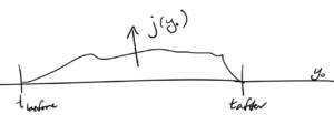
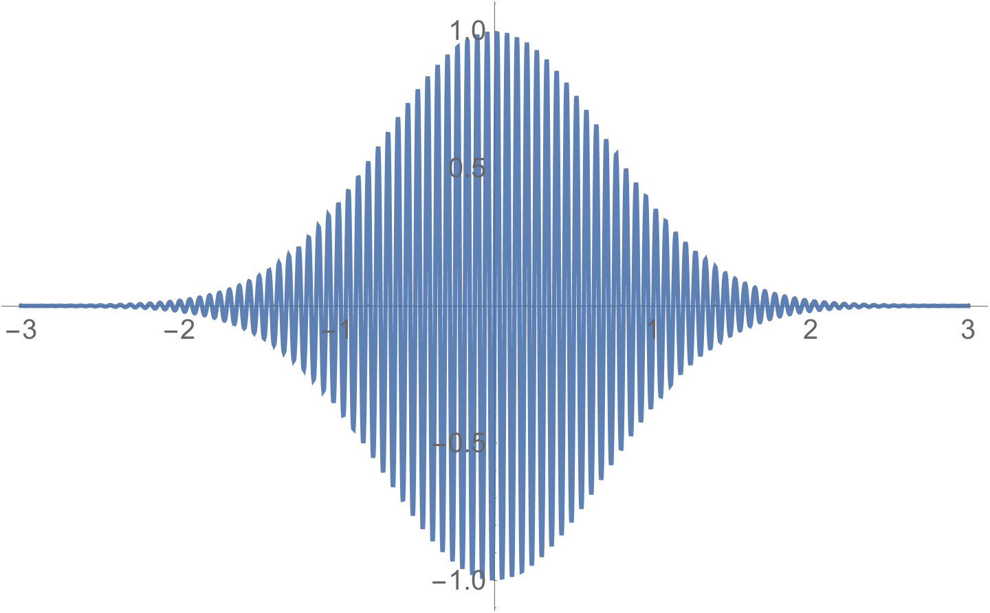
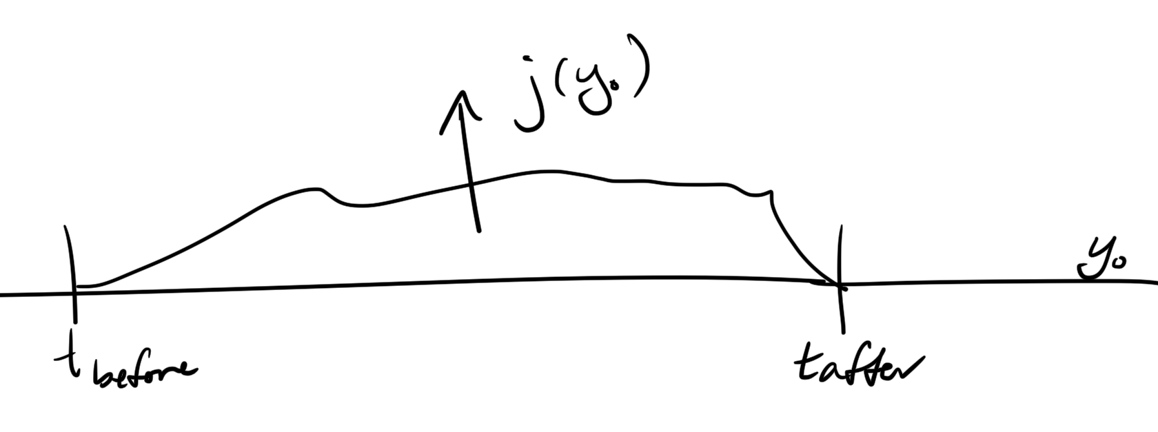
fig. 1. Finite window impulse response.

We imagined that we have a windowed source function \( j(y^0, \By) \), as sketched in fig. 1, which is acting as a forcing source for the non-homogeneous Klein-Gordon equation

\begin{equation}\label{eqn:qftLecture13:20}
\lr{ \partial_\mu \partial^\mu + m^2 } \phi = j
\end{equation}

Our solution was
\begin{equation}\label{eqn:qftLecture13:40}
\phi(x) = \phi(x_0) + i \int d^4 y D_R( x – y) j(y),
\end{equation}
where \( \phi(x_0) \) obeys the homogeneous equation, and
\begin{equation}\label{eqn:qftLecture13:60}
D_r(x – y) = \Theta(x^0 – y^0) \lr{ D(x – y) – D(y – x) },
\end{equation}
and \( D(x) = \int \frac{d^3 p}{(2\pi)^3 2 \omega_\Bp } \evalbar{ e^{-i p \cdot x} }{p^0 = \omega_\Bp} \) is the Weightmann function.

For \( x^0 > t_{\text{after}} \)
\begin{equation}\label{eqn:qftLecture13:80}
\phi(x)
=
\int \frac{d^3 p}{(2\pi)^3 \sqrt{ 2 \omega_\Bp }}
\evalbar{
\lr{ e^{-i p \cdot x} a_\Bp + e^{i p \cdot x } a_\Bp^\dagger }
}{
p^0 = \omega_\Bp
}
+ i
\int \frac{d^3 p}{(2\pi)^3 2 \omega_\Bp }
\evalbar{
\lr{ e^{-i p \cdot x} \tilde{j}(p) + e^{i p \cdot x} \tilde{j}(p_0, -\Bp) }
}{
p^0 = \omega_\Bp
}
\end{equation}
where we have used \( \tilde{j}^\conj(p_0, \Bp) = \tilde{j}(p_0, -\Bp) \). This gives
\begin{equation}\label{eqn:qftLecture13:100}
\phi(x) =
\int \frac{d^3 p}{(2\pi)^3 \sqrt{ 2 \omega_\Bp } }
\evalbar{
\lr{
e^{-i p \cdot x}
\lr{ a_\Bp + i \frac{\tilde{j}(p)}{\sqrt{2 \omega_\Bp}} }
+ e^{i p \cdot x }
\lr{ a_\Bp^\dagger – i \frac{\tilde{j}^\conj(p)}{\sqrt{2 \omega_\Bp}} }
}
}{
p^0 = \omega_\Bp
}
\end{equation}

It was left as an exercise to show that given
\begin{equation}\label{eqn:qftLecture13:120}
H = \int d^3 p \lr{ \inv{2} \pi^2 + \inv{2} \lr{ \spacegrad \phi}^2 + \frac{m^2}{2} \phi^2 },
\end{equation}
we obtain
\begin{equation}\label{eqn:qftLecture13:140}
H_{\text{after}} =
\int d^3 x \omega_\Bp
\lr{ a_\Bp^\dagger – i \frac{\tilde{j}^\conj(p)}{\sqrt{2 \omega_\Bp}} }
\lr{ a_\Bp + i \frac{\tilde{j}(p)}{\sqrt{2 \omega_\Bp}} }
\end{equation}

System in ground state
\begin{equation}\label{eqn:qftLecture13:160}
\bra{0} \hatH_{\text{before}} \ket{0} = \expectation{E}_{\text{before}} = 0.
\end{equation}
\begin{equation}\label{eqn:qftLecture13:180}
\begin{aligned}
\bra{0} \hatH_{\text{after}} \ket{0} = \expectation{E}_{\text{after}}
&=
\int d^3 x \omega_\Bp
\frac{ \tilde{j}^\conj(p) \tilde{j}(p)}{2 \omega_\Bp} \\
&=
\inv{2} \int d^3 x
\Abs{j(p)}^2.
\end{aligned}
\end{equation}
We can identify
\begin{equation}\label{eqn:qftLecture13:200}
N(\Bp) =
\frac{\Abs{j(p)}^2}{2 \omega_\Bp},
\end{equation}
as the number density of particles with momentum \( \Bp \).

Digression: coherent states.

Defintion: Coherent state.

A coherent state is an eigenstate of the destruction operator
\begin{equation*}
a \ket{\alpha} = \alpha \ket{\alpha}.
\end{equation*}

For the SHO, if we solve for such a coherent state, we find
\begin{equation}\label{eqn:qftLecture13:240}
\ket{\alpha} = \text{constant} \times \sum_{n = 0}^\infty \frac{\alpha^n}{n!} \lr{ a^\dagger }^n \ket{0}.
\end{equation}
If we assume the existence of a coherent state
\begin{equation}\label{eqn:qftLecture13:260}
a_\Bp \ket{
\frac{j(p)}{\sqrt{2 \omega_\Bp}}
}
=
\frac{j(p)}{\sqrt{2 \omega_\Bp}}
\ket{
\frac{j(p)}{\sqrt{2 \omega_\Bp}}
},
\end{equation}
then the expectation value of the number operator with respect to this state is the number density identified in \ref{eqn:qftLecture13:200}
\begin{equation}\label{eqn:qftLecture13:1200}
\bra{
\frac{j(p)}{\sqrt{2 \omega_\Bp}}
}
a_\Bp^\dagger a_\Bp
\ket{
\frac{j(p)}{\sqrt{2 \omega_\Bp}}
} = \frac{\Abs{j(p)}^2}{2 \omega_\Bp} = N(\Bp).
\end{equation}

Feynman’s Green’s function

\begin{equation}\label{eqn:qftLecture13:280}
\begin{aligned}
D_F(x)
&=
\Theta(x^0) D(x) +
\Theta(-x^0) D(-x) \\
&=
\Theta(x^0) \bra{0} \phi(x) \phi(0) \ket{0}
+\Theta(x^0) \bra{0} \phi(-x) \phi(0) \ket{0}
\end{aligned}
\end{equation}
Utilizing a translation operation \( U(a) = e^{i a_\mu P^\mu } \), where \( U(a) \phi(y) U^\dagger(a) = \phi(y + a) \), this second operation can be written as
\begin{equation}\label{eqn:qftLecture13:300}
\begin{aligned}
\bra{0} \phi(-x) \phi(0) \ket{0}
&=
\bra{0} U^\dagger(a) U(a) \phi(-x) U^\dagger(a) U(a) \phi(0) U^\dagger(a) U(a) \ket{0} \\
&=
\bra{0} U(a) \phi(-x) U^\dagger(a) U(a) \phi(0) U^\dagger(a) \ket{0} \\
&=
\bra{0} \phi(-x + a) \phi(a) \ket{0},
\end{aligned}
\end{equation}
In particular, with \( a = x \)
\begin{equation}\label{eqn:qftLecture13:320}
\bra{0} \phi(-x) \phi(0) \ket{0}
=
\bra{0} \phi(0) \phi(x) \ket{0},
\end{equation}
so the Feynman’s Green function can be written
\begin{equation}\label{eqn:qftLecture13:340}
D_F(x) =
\Theta(x^0) \bra{0} \phi(x) \phi(0) \ket{0}
+\Theta(x^0) \bra{0} \phi(x) \phi(x) \ket{0}
=
\bra{0}
\lr{
\Theta(x^0)
\phi(x) \phi(0)
+
\Theta(-x^0)
\phi(0) \phi(x)
}
\ket{0}.
\end{equation}
We define

Definition: Time ordered product.

The time ordered product of two operators is defined as
\begin{equation*}
T(\phi(x) \phi(y)) =
\left\{
\begin{array}{l l}
\phi(x)\phi(y) & \quad \mbox{\( x^0 > y^0 \)} \\
\phi(y)\phi(x) & \quad \mbox{\( x^0 < y^0 \)} \\
\end{array}
\right.,
\end{equation*}
or
\begin{equation*}
T(\phi(x) \phi(y)) =
\phi(x)\phi(y) \Theta(x^0 – y^0)
+
\phi(y)\phi(x) \Theta(y^0 – x^0).
\end{equation*}

Using this helpful construct, the Feynman’s Green function can now be written in a very simple fashion
\begin{equation}\label{eqn:qftLecture13:380}
\boxed{
D_F(x) = \bra{0} T(\phi(x) \phi(0)) \ket{0}.
}
\end{equation}

Remark:

Recall that the four dimensional form of the Green’s function was
\begin{equation}\label{eqn:qftLecture13:400}
D_F = i \int \frac{d^4 p}{(2 \pi)^4} e^{-i p \cdot x} \inv{ p^2 – m^2 }.
\end{equation}
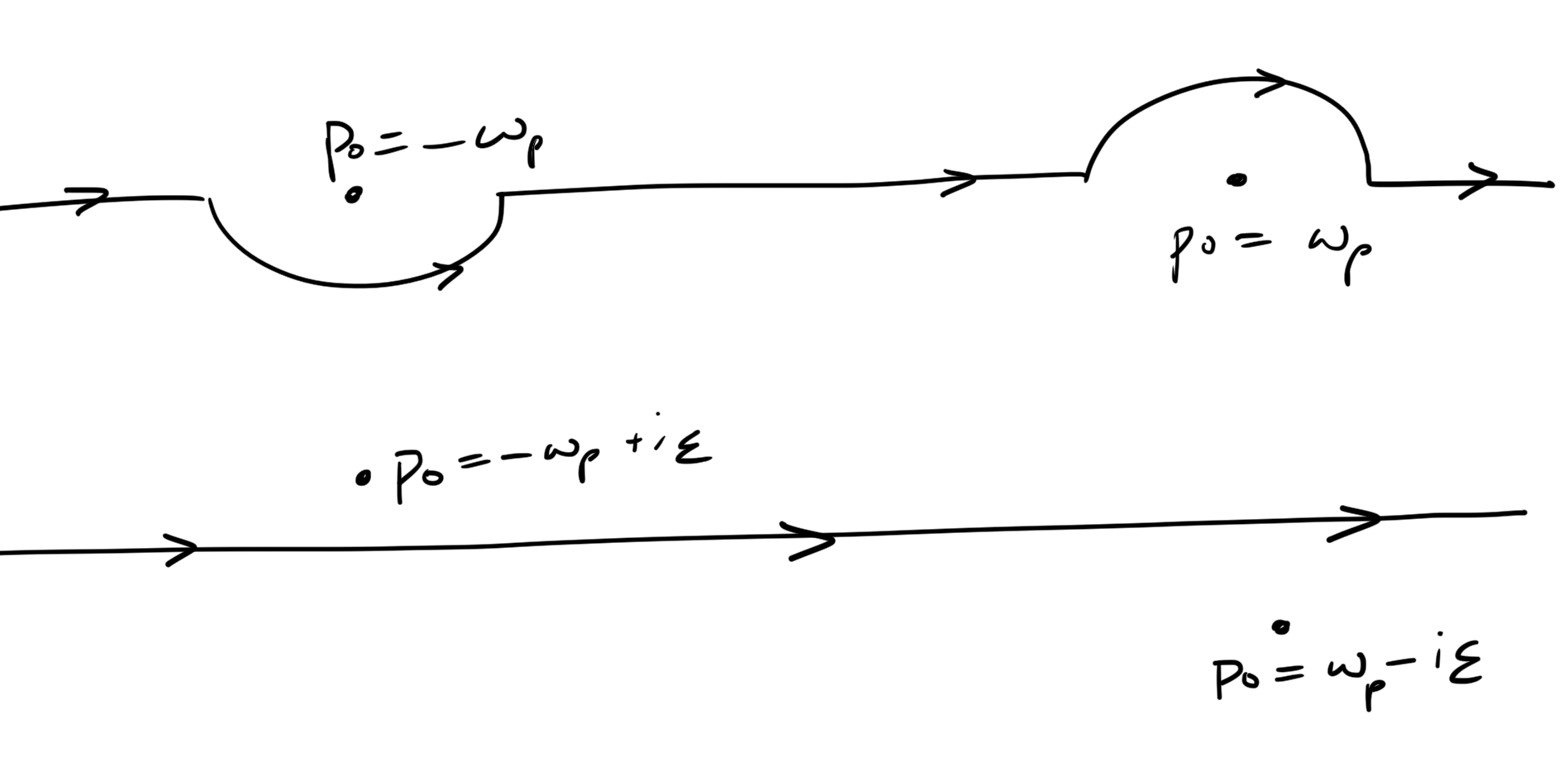
For the Feynman case, the contour that we were taking around the poles can also be accomplished by shifting the poles strategically, as sketched in fig. 2.

fig. 2. Feynman deformation or equivalent shift of the poles.


This shift can be expressed explicit algebraically by introducing an offset
\begin{equation}\label{eqn:qftLecture13:420}
D_F = i \int \frac{d^4 p}{(2 \pi)^4} e^{-i p \cdot x} \inv{ p^2 – m^2 + i \epsilon }
\end{equation}
which puts the poles at

\begin{equation}\label{eqn:qftLecture13:440}
\begin{aligned}
p^0
&= \pm \sqrt{ \omega_\Bp – i \epsilon } \\
&= \pm \omega_\Bp \lr{ 1 – \frac{i \epsilon}{\omega_\Bp^2} }^{1/2} \\
&= \pm \omega_\Bp \lr{ 1 – \inv{2} \frac{i \epsilon}{\omega_\Bp^2} } \\
&=
\left\{
\begin{array}{l}
+\omega_\Bp – \inv{2} i \frac{\epsilon}{\omega_\Bp} \\
-\omega_\Bp + \inv{2} i \frac{\epsilon}{\omega_\Bp} \\
\end{array}
\right.
\end{aligned}
\end{equation}


Interacting field theory: perturbation theory in QFT.

We perturb the Hamiltonian
\begin{equation}\label{eqn:qftLecture13:500}
H = H_0 + H_{\text{int}}
\end{equation}
where \( H_0 \) is the free Hamiltonian and \( H_{\text{int}} \) is the interaction term (the perturbation).

Example:

\begin{equation}\label{eqn:qftLecture13:460}
\begin{aligned}
H_0 &= SHO = \frac{p^2}{2} + \frac{\omega^2 q^2}{2} \\
H_{\text{int}} &= \lambda q^4,
\end{aligned}
\end{equation}
i.e. the anharmonic oscillator.

In QFT
\begin{equation}\label{eqn:qftLecture13:480}
\begin{aligned}
H_0 &=
\int d^3 x \lr{ \inv{2} \pi^2 + \inv{2} \lr{ \spacegrad \phi}^2 + \frac{m^2}{2} \phi^2 } \\
H_{\text{int}} &=
\lambda \int d^3 x \phi^4.
\end{aligned}
\end{equation}

We will expand the interaction in small \( \lambda \). Perturbation theory is the expansion in a small dimensionless coupling constant, such as

  • \( \lambda \) in \( \lambda \phi^4 \) theory,
  • \( \alpha = e^2/4 \pi \sim \inv{137} \) in QED, and
  • \( \alpha_s \) in QCD.

Perturbation theory, interaction representation and Dyson formula

\begin{equation}\label{eqn:qftLecture13:520}
H = H_0 + H_{\text{int}}
\end{equation}
Example interaction
\begin{equation}\label{eqn:qftLecture13:540}
H_{\text{int}} = \lambda \int d^3 x \phi^4
\end{equation}

We know all there is to know about \( H_0 \) (decoupled SHOs, …)
\begin{equation}\label{eqn:qftLecture13:560}
H_0 \ket{0} = \ket{0} E^0_{\text{vac}}
\end{equation}
where \( E^0_{\text{vac}} = 0 \). Assume
\begin{equation}\label{eqn:qftLecture13:580}
\lr{ H_0 + H_{\text{int}} } \ket{\Omega} = \ket{\Omega} E_{\text{vac}},
\end{equation}
where the ground state energy of the perturbed system is zero when \( \lambda = 0 \). That is \( E_{\text{vac}}(\lambda = 0 ) = 0 \).

So for
\begin{equation}\label{eqn:qftLecture13:600}
\evalbar{\phi(x) }{x^0 = t_0, \text{some fixed value}}
=
\int \frac{d^3}{(2 \pi)^3 \sqrt{ 2 \omega_\Bp } }
\evalbar{
\lr{
e^{-i p \cdot x} a_\Bp
+ e^{i p \cdot x} a_\Bp^\dagger }
}
{
p^0 = \omega_\Bp
}.
\end{equation}
Let’s call \( \phi(\Bx, t_0) \) the free Schr\”{o}dinger operator, where
\( \phi(\Bx, t_0) \) is evaluated at a fixed value of \( t_0 \). At such a point, the Schr\”{o}dinger and Heisenberg pictures coincide.
\begin{equation}\label{eqn:qftLecture13:620}
\antisymmetric{\phi(\Bx, t_0)}{\pi(\By, t_0)} = i \delta^3(\Bx – \By).
\end{equation}

Normally (QM) one defines the Heisenberg operator as
\begin{equation}\label{eqn:qftLecture13:640}
O_H = e^{i H(t – t_0)} O_S e^{-i H(t – t_0)},
\end{equation}
where \( O_H \) depends on time, and \( O_S \) is defined at a fixed time \( t_0 \), usually 0.
From \ref{eqn:qftLecture13:640} we find
\begin{equation}\label{eqn:qftLecture13:660}
\ddt{O_H} = i \antisymmetric{H}{O_H}.
\end{equation}
The equivalent of \ref{eqn:qftLecture13:640} in QFT is very complicated. We’d like to develop an intermediate picture.

We will define an intermediate picture, called the “interaction representation”, which is equivalent to the Heisenberg picture with respect to \( H_0 \).

Definition: Intermediate picture operator.

\begin{equation*}
\phi_I(t, \Bx) =
e^{i H_0(t – t_0) }
\phi(t_0, \Bx)
e^{-i H_0(t – t_0) }.
\end{equation*}

This is familiar, and is the Heisenberg picture operator that we had in free QFT
\begin{equation}\label{eqn:qftLecture13:700}
\phi_I(t, \Bx) =
\int \frac{d^3}{(2 \pi)^3 \sqrt{ 2 \omega_\Bp } }
\evalbar{
\lr{
e^{-i p \cdot x} a_\Bp
+ e^{i p \cdot x} a_\Bp^\dagger }
}
{
p^0 = \omega_\Bp
},
\end{equation}
where \( x_0 = t \).

The Heisenberg picture operator is
\begin{equation}\label{eqn:qftLecture13:720}
\begin{aligned}
\phi_H(t, \Bx)
&=
\phi(t, \Bx) \\
&=
e^{i H(t – t_0) }
e^{-i H_0(t – t_0) }
\lr{
e^{i H_0(t – t_0) }
\phi_S(t_0, \Bx)
e^{-i H_0(t – t_0) }
}
e^{i H_0(t – t_0) }
e^{-i H(t – t_0) } \\
&=
e^{i H(t – t_0) }
e^{-i H_0(t – t_0) }
\phi_I(t, \Bx)
e^{-i H_0(t – t_0) }
e^{i H(t – t_0) }
\end{aligned}
\end{equation}
or
\begin{equation}\label{eqn:qftLecture13:760}
\phi_H(t, \Bx)
=
U^\dagger(t, t_0)
\phi_I(t_0, \Bx)
U(t, t_0),
\end{equation}
where
\begin{equation}\label{eqn:qftLecture13:740}
U(t, t_0) =
e^{i H_0(t – t_0) }
e^{-i H(t – t_0) }.
\end{equation}

We want to apply perturbation techniques to find \( U(t, t_0) \) which is complicated.

\begin{equation}\label{eqn:qftLecture13:780}
\begin{aligned}
i \PD{t}{} U(t, t_0)
&=
i e^{i H_0(t – t_0) } i H_0
e^{-i H(t – t_0) }
+
i e^{i H_0(t – t_0) }
e^{-i H(t – t_0) } (-i H) \\
&=
e^{i H_0(t – t_0) }
\lr{ -H_0 + H }
e^{-i H(t – t_0) } \\
&=
e^{i H_0(t – t_0) }
H_{\text{int}}
e^{-i H_0(t – t_0) }
e^{i H_0(t – t_0) }
e^{-i H(t – t_0) }
\end{aligned}
\end{equation}
so we have
\begin{equation}\label{eqn:qftLecture13:800}
\boxed{
i \PD{t}{} U(t, t_0)
=
H_{\text{int}, I}(t) U(t, t_0).
}
\end{equation}
For the (Schr\”{o}dinger) interaction \( H_{\text{int}} = \
\lambda \int d^3 x \phi^4(\Bx, t_0) \), what we really mean by
\( H_{\text{int}, I}(t) \) is
\begin{equation}\label{eqn:qftLecture13:820}
H_{\text{int}, I}(t) = \lambda \int d^3 x \phi_I^4(\Bx, t).
\end{equation}

It will be more convenient to remove the explicit \( \lambda \) factor from the interaction Hamiltonian, and write instead
\begin{equation}\label{eqn:qftLecture13:880}
H_{\text{int}, I}(t) = \int d^3 x \phi_I^4(\Bx, t),
\end{equation}
so the equation to solve is
\begin{equation}\label{eqn:qftLecture13:1220}
i \PD{t}{} U(t, t_0)
=
\lambda H_{\text{int}, I}(t) U(t, t_0).
\end{equation}

We assume that
\begin{equation}\label{eqn:qftLecture13:900}
U(t, t_0)
=
U_0(t, t_0)
+ \lambda U_1(t, t_0)
+ \lambda^2 U_2(t, t_0)
+ \cdots
+ \lambda^n U_n(t, t_0)
\end{equation}

Plugging into \ref{eqn:qftLecture13:880} we have
\begin{equation}\label{eqn:qftLecture13:1160}
\begin{aligned}
i &\lambda^0 \PD{t}{}U_0(t, t_0)
+ i \lambda^1 \PD{t}{}U_1(t, t_0)
+ i \lambda^2 \PD{t}{}U_2(t, t_0)
+ \cdots
+ i \lambda^n \PD{t}{}U_n(t, t_0) \\
&=
\lambda H_{\text{int}, I}(t)
\lr{
1
+ \lambda U_1(t, t_0)
+ \lambda^2 U_2(t, t_0)
+ \cdots
+ \lambda^n U_n(t, t_0)
},
\end{aligned},
\end{equation}
so
equating equal powers of \( \lambda \) on each side gives a recurrence relation for each \( U_k, k > 0 \)
\begin{equation}\label{eqn:qftLecture13:1180}
\PD{t}{}U_k(t, t_0) = -i H_{\text{int}, I}(t) U_{k-1}(t, t_0).
\end{equation}

Let’s consider each power in turn.

\(O(\lambda^0)\):

Solving \ref{eqn:qftLecture13:800} to \( O(\lambda^0) \) gives
\begin{equation}\label{eqn:qftLecture13:840}
i \PD{t}{} U_0(t, t_0) = 0,
\end{equation}
or
\begin{equation}\label{eqn:qftLecture13:860}
U(t, t_0) = 1 + O(\lambda).
\end{equation}

\(O(\lambda^1)\):

\begin{equation}\label{eqn:qftLecture13:940}
\PD{t}{U_1(t, t_0)} = -i H_{\text{int}, I}(t),
\end{equation}
which has solution
\begin{equation}\label{eqn:qftLecture13:960}
U_1(t, t_0) = -i \int_{t_0}^t H_{\text{int}, I}(t’) dt’.
\end{equation}

\(O(\lambda^2)\):

\begin{equation}\label{eqn:qftLecture13:1000}
\begin{aligned}
\PD{t}{U_2(t, t_0)}
&= -i H_{\text{int}, I}(t) U_1(t, t_0) \\
&= (-i)^2 H_{\text{int}, I}(t)
\int_{t_0}^t H_{\text{int}, I}(t’) dt’,
\end{aligned}
\end{equation}
which has solution
\begin{equation}\label{eqn:qftLecture13:1020}
\begin{aligned}
U_2(t, t_0)
&= (-i )^2
\int_{t_0}^t H_{\text{int}, I}(t”) dt”
\int_{t_0}^{t”} H_{\text{int}, I}(t’) dt’ \\
&= (-i )^2
\int_{t_0}^t dt”
\int_{t_0}^{t”}
dt’
H_{\text{int}, I}(t”)
H_{\text{int}, I}(t’).
\end{aligned}
\end{equation}

\(O(\lambda^3)\):

\begin{equation}\label{eqn:qftLecture13:1060}
\PD{t}{U_3(t, t_0)}
=
-i
H_{\text{int}, I}(t) U_2(t, t_0)
\end{equation}
so
\begin{equation}\label{eqn:qftLecture13:1240}
\begin{aligned}
U_3(t, t_0)
&=
-i
\int_{t_0}^t dt”’
H_{\text{int}, I}(t”’) U_2(t”’, t_0) \\
&=
(-i )^3
\int_{t_0}^t dt”’
H_{\text{int}, I}(t”’)
\int_{t_0}^{t”’} dt”
\int_{t_0}^{t”}
dt’
H_{\text{int}, I}(t”)
H_{\text{int}, I}(t’) \\
&=
(-i)^3
\int_{t_0}^t dt”’
\int_{t_0}^{t”’} dt”
\int_{t_0}^{t”} dt’
H_{\text{int}, I}(t”’)
H_{\text{int}, I}(t”)
H_{\text{int}, I}(t’)
\end{aligned}
\end{equation}

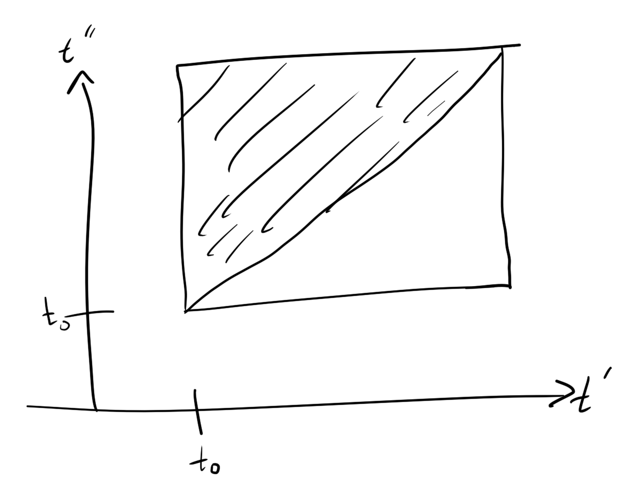
Simplifying the integration region.

For the two fold integral, the integration range is the upper triangular region sketched in fig. 3.

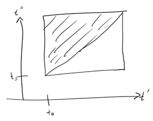
fig. 3. Upper triangular integration region.

Claim:

We can integrate over the entire square, and divide by two, provided we keep the time ordering
\begin{equation}\label{eqn:qftLecture13:1040}
U_2(t, t_0)
= \frac{(-i )^2}{2}
\int_{t_0}^t dt”
\int_{t_0}^{t”}
dt’
T(H_{\text{int}, I}(t”) H_{\text{int}, I}(t’) )
\end{equation}

Demonstration:
\begin{equation}\label{eqn:qftLecture13:1100}
\begin{aligned}
\frac{(-i)^2}{2}
&\int_{t_0}^t dt”
\int_{t_0}^t dt’
T( H_I(t”) H_I(t’) ) \\
&=
\frac{(-i)^2}{2}
\int_{t_0}^t dt”
\int_{t_0}^t dt’
\Theta(t”- t’)
H_I(t”) H_I(t’)
+
\frac{(-i)^2}{2}
\int_{t_0}^t dt”
\int_{t_0}^t dt’
\Theta(t’- t”)
H_I(t’) H_I(t”),
\end{aligned}
\end{equation}
but the \( \Theta(t” – t’) \) function is non-zero only for \( t” – t’ > 0 \), or \( t’ < t” \), and the \( \Theta(t’ – t”) \) function is non-zero only for \( t’ – t” > 0 \), or \( t” < t’ \), so we can adjust the integration ranges for
\begin{equation}\label{eqn:qftLecture13:1260}
\begin{aligned}
\frac{(-i)^2}{2}
&\int_{t_0}^t dt”
\int_{t_0}^t dt’
T( H_I(t”) H_I(t’) ) \\
&=
\frac{(-i)^2}{2}
\int_{t_0}^t dt”
\int_{t_0}^{t”} dt’
H_I(t”) H_I(t’)
+
\frac{(-i)^2}{2}
\int_{t_0}^{t’} dt”
\int_{t_0}^t dt’
H_I(t’) H_I(t”) \\
&=
\frac{(-i)^2}{2}
\int_{t_0}^t dt”
\int_{t_0}^{t”} dt’
H_I(t”) H_I(t’)
+
\frac{(-i)^2}{2}
\int_{t_0}^t dt”
\int_{t_0}^{t”} dt’
H_I(t”) H_I(t’) \\
&=
U_2(t, t_0),
\end{aligned}
\end{equation}
where we swapped integration variables in second integral. We can clearly do the same thing for the higher order repeated integrals, but instead of a \(1/2 = 1/2!\) adjustment for the number of orderings, we will require a \( 1/n! \) adjustment for an \( n \)-fold integral.

Summary:

\begin{equation}\label{eqn:qftLecture13:1120}
\begin{aligned}
U_0 &= 1 \\
U_1 &= -i \int_{t_0}^t dt_1 H_I(t_1) \\
U_2 &= \frac{(-i)^2}{2}
\int_{t_0}^t dt_1
\int_{t_0}^t dt_2
T( H_I(t_1)
H_I(t_2) ) \\
U_3 &= \frac{(-i)^3}{3!}
\int_{t_0}^t dt_1
\int_{t_0}^t dt_2
\int_{t_0}^t dt_3
T( H_I(t_1)
H_I(t_2)
H_I(t_3)
) \\
U_n &= \frac{(-i)^n}{n!}
\int_{t_0}^t dt_1
\int_{t_0}^t dt_2
\int_{t_0}^t dt_3
\cdots
\int_{t_0}^t dt_n
T( H_I(t_1)
H_I(t_2)
\cdots
H_I(t_n)
) \\
\end{aligned}
\end{equation}

Summing we find
\begin{equation}\label{eqn:qftLecture13:1140}
\begin{aligned}
U(t, t_0)
&= T \exp\lr{-i
\int_{t_0}^t dt_1 H_I(t’)
} \\
&=
\sum_{n = 0}^\infty
\frac{(-i)^n}{n!} \int_{t_0}^t dt_1 \cdots dt_n T( H_I(t_1) \cdots H_I(t_n) ).
\end{aligned}
\end{equation}

This is called Dyson’s formula.

Next time.

Our goal is to compute: \( \bra{\Omega} T(\phi(x_1) \cdots \phi(x_n)) \ket{\Omega} \).