[Click here for a PDF of this post with nicer formatting]
DISCLAIMER: Very rough notes from class. Some additional side notes, but otherwise barely edited.
What is a field?
A field is a map from space(time) to some set of numbers. These set of numbers may be organized some how, possibly scalars, or vectors, …
One example is the familiar spacetime vector, where \( \Bx \in \mathbb{R}^{d} \)
\begin{equation}\label{eqn:qftLecture1:20}
(\Bx, t) \rightarrow \mathbb{R}^{\lr{d,1}}
\end{equation}
Examples of fields:
- \( 0 + 1 \) dimensional “QFT”, where the spatial dimension is zero dimensional and we have one time dimension. Fields in this case are just functions of time \( x(t) \). That is, particle mechanics is a 0 + 1 dimensional classical field theory. We know that classical mechanics is described by the action
\begin{equation}\label{eqn:qftLecture1:40}
S = \frac{m}{2} \int dt \xdot^2.
\end{equation}
This is non-relativistic. We can make this relativistic by saying this is the first order term in the Taylor expansion
\begin{equation}\label{eqn:qftLecture1:60}
S = – m c^2 \int dt \sqrt{ 1 – \xdot^2/c^2 }.
\end{equation}
Classical field theory (of \( x(t) \)). The “QFT” of \( x(t) \). i.e. QM.
All of you know quantum mechanics. If you don’t just leave. Not this way (pointing to the window), but this way (pointing to the door).
The solution of a quantum mechanical state is
\begin{equation}\label{eqn:qftLecture1:80}
\bra{x} e^{-i H t/\,\hbar } \ket{x’},
\end{equation}
which can be found by evaluating the “Feynman path integral”
\begin{equation}\label{eqn:qftLecture1:100}
\sum_{\text{all paths x}} e^{i S[x]/\,\hbar}
\end{equation}
This will be particularly useful for QFT, despite the fact that such a sum is really hard to evaluate (try it for the Hydrogen atom for example). - \( 3 + 0 \) dimensional field theory, where we have 3 spatial dimensions and 0 time dimensions. Classical equilibrium static systems. The field may have a structure like
\begin{equation}\label{eqn:qftLecture1:120}
\Bx \rightarrow \BM(\Bx),
\end{equation}
for example, magnetization.
We can write the solution to such a system using the partition function
\begin{equation}\label{eqn:qftLecture1:140}
Z \sim \sum_{\text{all} \BM(x)} e^{-E[\BM]/\kB T}.
\end{equation}
For such a system the energy function may be like
\begin{equation}\label{eqn:qftLecture1:160}
E[\BM] = \int d^3 \Bx \lr{ a \BM^2(\Bx) + b \BM^4(\Bx) + c \sum_{i = 1}^3 \lr{ \PD{x_i}{} \BM }
\cdot \lr{ \PD{x_i}{} \BM }
}.
\end{equation}
There is an analogy between the partition function and the Feynman path integral, as both are summing over all possible energy states in both cases.
This will be probably be the last time that we mention the partition function and condensed matter physics in this term for this class. - \( 3 + 1 \) dimensional field theories, with 3 spatial dimensions and 1 time dimension.
Example, electromagnetism with \( \BE(\Bx, t), \BB(\Bx, t) \) or better use \( \BA(\Bx, t), \phi(\Bx, t) \). The action is
\begin{equation}\label{eqn:qftLecture1:180}
S = -\inv{16 \pi c} \int d^3 \Bx dt \lr{ \BE^2 – \BB^2 }.
\end{equation}
This is our first example of a relativistic field theory in \( 3 + 1 \) dimensions. It will take us a while to get there.
These are examples of classical field theories, such as fluid dynamics and general relativity. We want to consider electromagnetism because this is the place that we everything starts to fall apart (i.e. blackbody radiation, relating to the equilibrium states of radiating matter). Part of the resolution of this was the quantization of the energy states, where we studied the normal modes of electromagnetic radiation in a box. These modes can be considered an infinite number of radiating oscillators (the ultraviolet catastrophe). This was resolved by Planck by requiring those energy states to be quantized (an excellent discussion of this can be found in [1]. In that sense you have already seen quantum field theory.
For electromagnetism the classical description is not always good. Examples:
- blackbody radiation.
- electron energy \( e^2/r_\txte \) of a point charge diverges as \( r_\txte \rightarrow 0 \).
We can define the classical radius of the electron by
\begin{equation}\label{eqn:qftLecture1:200}
\frac{e^2}{r^{\textrm{cl}}_{\txte}} \sim m_\txte c^2,
\end{equation}
or
\begin{equation}\label{eqn:qftLecture1:220}
r^{\textrm{cl}}_{\txte} \sim \frac{m_\txte c^2}{e^2} \sim 10^{-15} \text{m}
\end{equation}
Don’t treat this very seriously, but it becomes useful at frequencies \( \omega \sim c/r_\txte \), where \( r_\txte/c \) is approximately the time for light to cross a distance \( r_\txte \).
At frequencies like this, we should not believe the solutions that are obtained by classical electrodynamics.
In particular, self-accelerating solutions appear at these frequencies in classical EM. This is approximately \( \omega_\conj \sim 10^{23} Hz \), or
\begin{equation}\label{eqn:qftLecture1:240}
\begin{aligned}
\,\hbar \omega_\conj
&\sim \lr{ 10^{-21} \,\text{MeV s}} \lr{ 10^{23} \,\text{1/s} }\\
&\sim 100 \text{MeV}.
\end{aligned}
\end{equation}
At such frequencies particle creation becomes possible.
Scales
A (dimensionless) value that is very useful in determining scale is
\begin{equation}\label{eqn:qftLecture1:260}
\alpha = \frac{e^2}{4 \pi \,\hbar c} \sim \inv{137},
\end{equation}
called the fine scale constant, which relates three important scales relevant to quantum mechanics, as sketched in fig. 1.
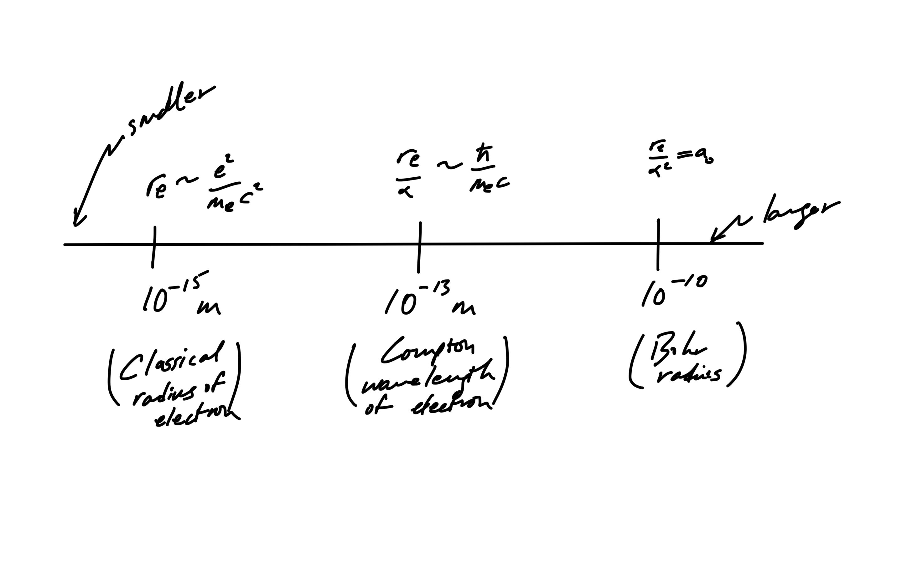
fig. 1. Interesting scales in quantum mechanics.
- The Bohr radius (large end of the scale).
- The Compton wavelength of the electron.
- The classical radius of the electron.
Bohr radius
A quick motivation for the Bohr radius was mentioned in passing in class while discussing scale, following the high school method of deriving the Balmer series ([2]).
That method assumes a circular electron trajectory (\(i = \Be_1 \Be_2\))
\begin{equation}\label{eqn:qftLecture1:280}
\begin{aligned}
\Br &= r \Be_1 e^{i \omega t} \\
\Bv &= \omega r \Be_2 e^{i \omega t} \\
\Ba &= -\omega^2 r \Be_1 e^{i \omega t} \\
\end{aligned}
\end{equation}
The Coulomb force (in cgs units) on the electron is
\begin{equation}\label{eqn:qftLecture1:300}
\BF = m\Ba = -m \omega^2 r \Be_1 e^{i \omega t} = \frac{-e (e)}{r^2} \Be_1 e^{i \omega t},
\end{equation}
or
\begin{equation}\label{eqn:qftLecture1:320}
m \lr{ \frac{v}{r}}^2 r = \frac{e^2}{r^2},
\end{equation}
giving
\begin{equation}\label{eqn:qftLecture1:340}
m v^2 = \frac{e^2}{r}.
\end{equation}
The energy of the system, including both Kinetic and potential (from an infinite reference point) is
\begin{equation}\label{eqn:qftLecture1:360}
\begin{aligned}
E
&= \inv{2} m v^2 – \frac{e^2}{r} \\
&= – \inv{2} m v^2 \sim \,\hbar \omega = \,\hbar \frac{v}{r},
\end{aligned}
\end{equation}
or
\begin{equation}\label{eqn:qftLecture1:380}
m v r \sim \,\hbar.
\end{equation}
Eliminating \( v \) using \ref{eqn:qftLecture1:340}, assuming a ground state radius \( r = a_0 \) gives
\begin{equation}\label{eqn:qftLecture1:400}
a_0 \sim \frac{\hbar^2}{m e^2}.
\end{equation}
The Bohr radius is of the order \( 10^{-10} \text{m} \).
Compton wavelength.
When particle momentum starts approaching the speed of light, by the uncertainty relation (\(\Delta x \Delta p \sim \,\hbar\)) the variation in position must be of the order
\begin{equation}\label{eqn:qftLecture1:420}
\lambda_\txtc \sim \frac{\hbar}{m_\txte c},
\end{equation}
called the Compton wavelength.
Similarly, when the length scales are reduced to the Compton wavelength, the momentum increases to relativistic levels.
Because of the relativistic velocities at the Compton wavelength, particle creation and annihilation occurs and any theory has to account for multiple particle states.
Relations.
Scaling the Bohr radius once by the fine structure constant, we obtain the Compton wavelength (after dropping factors of \( 4\pi \))
\begin{equation}\label{eqn:qftLecture1:440}
\begin{aligned}
a_0 \alpha
&= \frac{\hbar^2}{m e^2}
\frac{e^2}{4 \pi \,\hbar c} \\
&= \frac{\hbar}{4 \pi m c} \\
&\sim
\frac{\hbar}{m c} \\
&= \lambda_\txtc.
\end{aligned}
\end{equation}
Scaling once more, we obtain (after dropping another \( 4\pi\)) the classical electron radius
\begin{equation}\label{eqn:qftLecture1:n}
\begin{aligned}
\lambda_\txtc \alpha
&=
\frac{e^2}{4 \pi m c^2} \\
&\sim
\frac{e^2}{m c^2}.
\end{aligned}
\end{equation}
References
[1] D. Bohm. Quantum Theory. Courier Dover Publications, 1989.
[2] A.P. French and E.F. Taylor. An Introduction to Quantum Physics. CRC Press, 1998.