math and physics play

ECE1505H Convex Optimization. Lecture 4: Sets and convexity. Taught by Prof. Stark Draper

January 25, 2017 ece1505 , , , , , , ,

ECE1505H Convex Optimization. Lecture 4: Sets and convexity. Taught by Prof. Stark Draper

[Click here for a PDF of this post with nicer formatting]

Disclaimer

Peeter’s lecture notes from class. These may be incoherent and rough.

These are notes for the UofT course ECE1505H, Convex Optimization, taught by Prof. Stark Draper, covering [1] content.

Today

  • more on various sets: hyperplanes, half-spaces, polyhedra, balls, ellipses, norm balls, cone of PSD
  • generalize inequalities
  • operations that preserve convexity
  • separating and supporting hyperplanes.
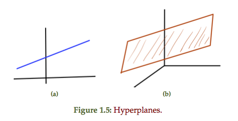
Hyperplanes

Find some \( \Bx_0 \in \mathbb{R}^n \) such that \( \Ba^\T \Bx_0 = \Bb \), so

\begin{equation}\label{eqn:convexOptimizationLecture4:20}
\begin{aligned}
\setlr{ \Bx | \Ba^\T \Bx = \Bb }
&=
\setlr{ \Bx | \Ba^\T \Bx = \Ba^\T \Bx_0 } \\
&=
\setlr{ \Bx | \Ba^\T (\Bx – \Bx_0) } \\
&=
\Bx_0 + \Ba^\perp,
\end{aligned}
\end{equation}

where

\begin{equation}\label{eqn:convexOptimizationLecture4:40}
\Ba^\perp = \setlr{ \Bv | \Ba^\T \Bv = 0 }.
\end{equation}

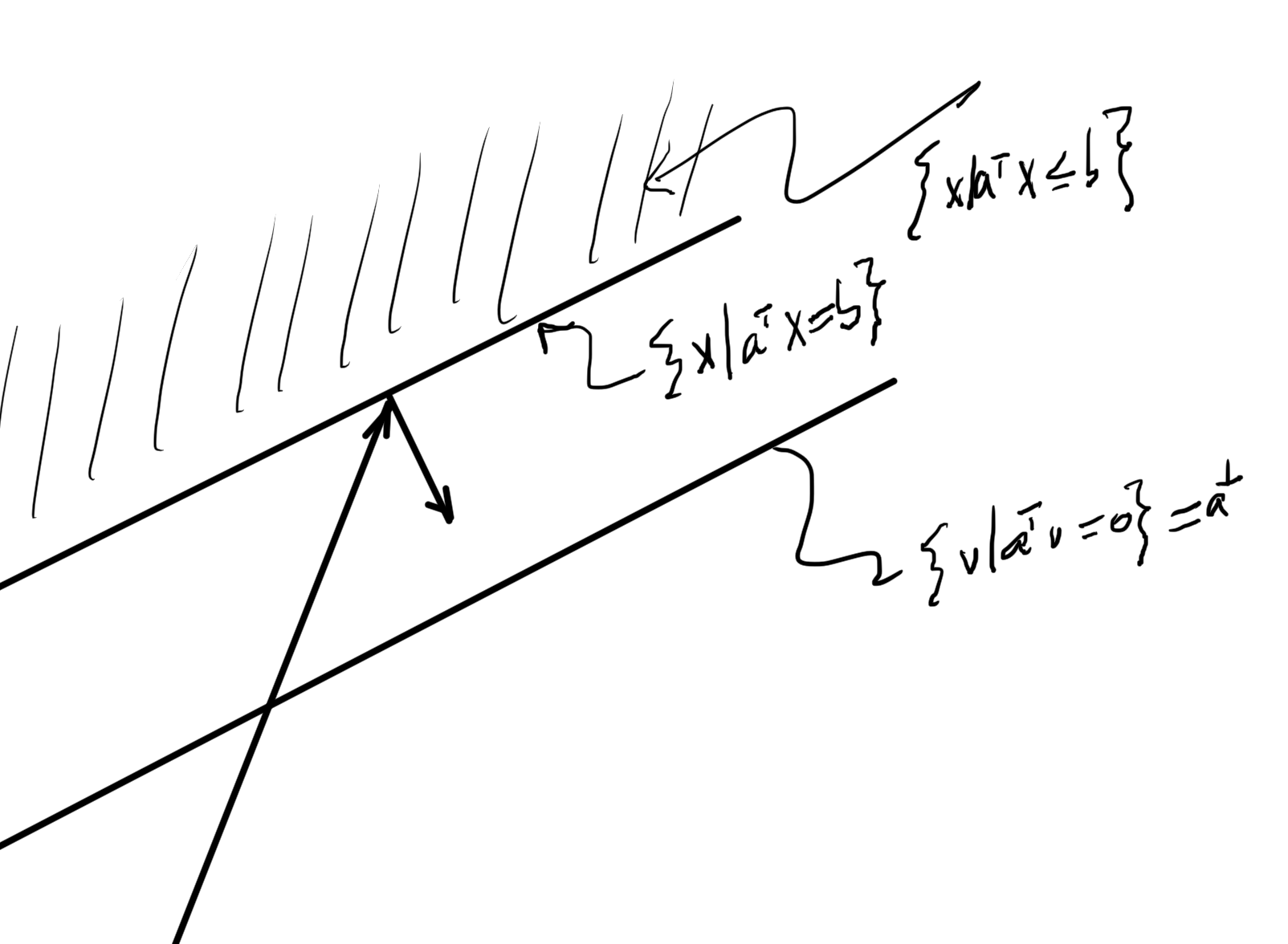
fig. 1. Parallel hyperplanes.
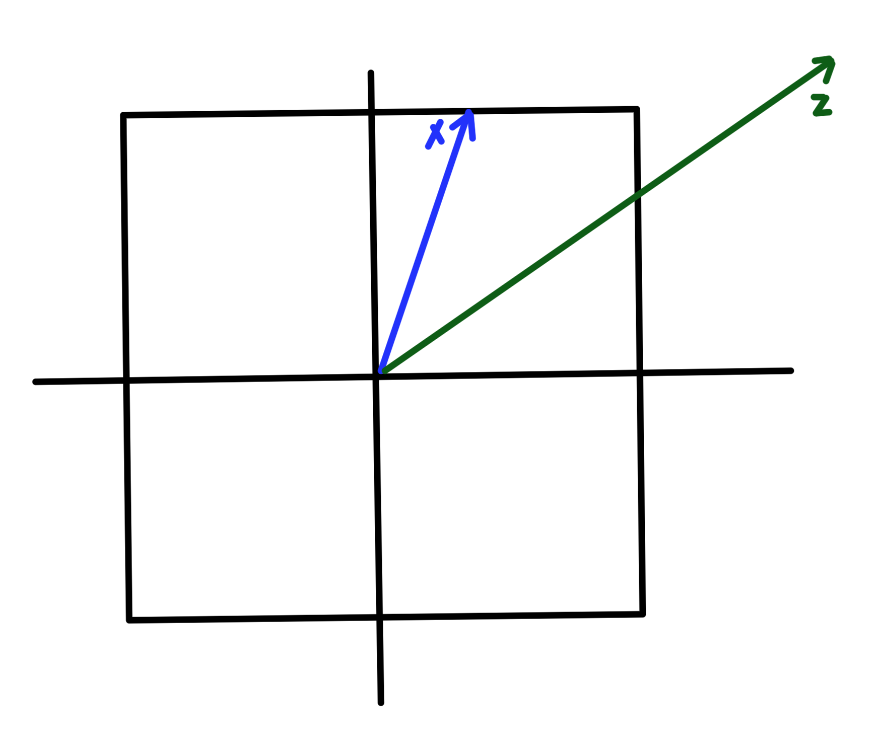
 

Recall

\begin{equation}\label{eqn:convexOptimizationLecture4:60}
\Norm{\Bz}_\conj = \sup_\Bx \setlr{ \Bz^\T \Bx | \Norm{\Bx} \le 1 }
\end{equation}

Denote the optimizer of above as \( \Bx^\conj \). By definition

\begin{equation}\label{eqn:convexOptimizationLecture4:80}
\Bz^\T \Bx^\conj \ge \Bz^\T \Bx \quad \forall \Bx, \Norm{\Bx} \le 1
\end{equation}

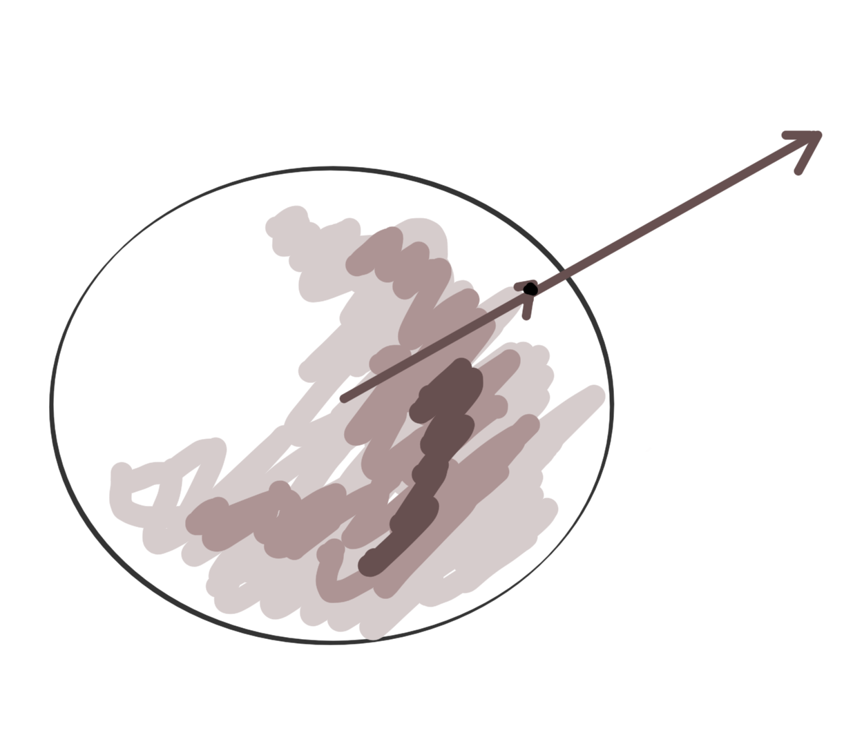
This defines a half space in which the unit ball

\begin{equation}\label{eqn:convexOptimizationLecture4:100}
\setlr{ \Bx | \Bz^\T (\Bx – \Bx^\conj \le 0 }
\end{equation}

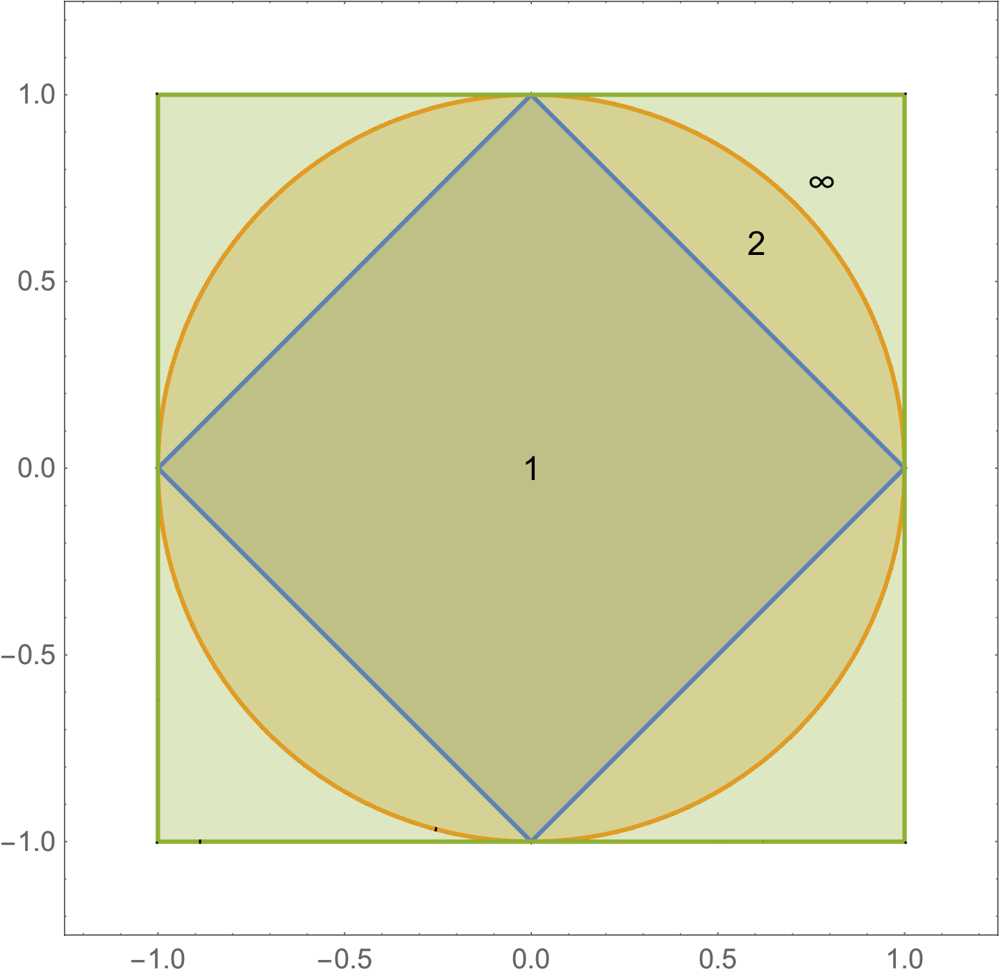
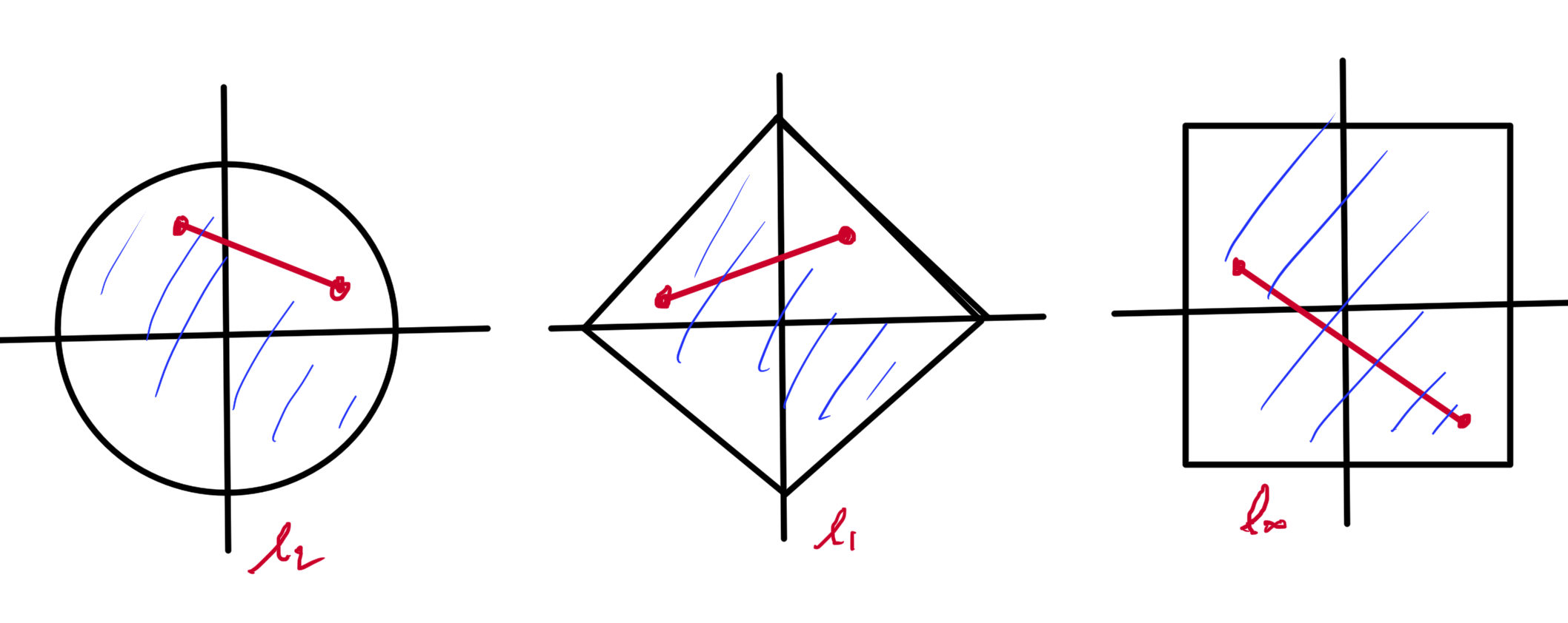
Start with the \( l_1 \) norm, duals of \( l_1 \) is \( l_\infty \)


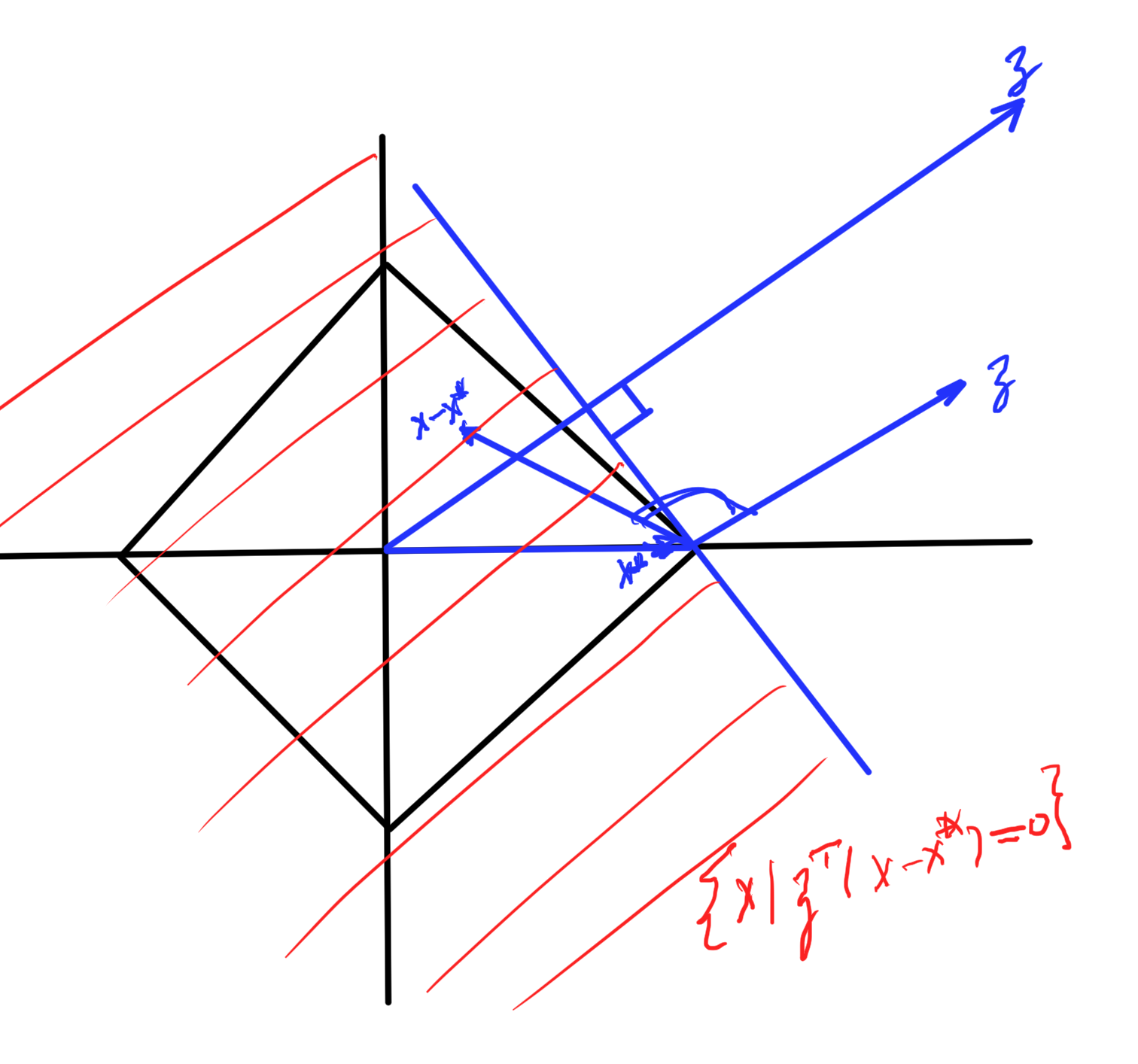
fig. 2. Half space containing unit ball.

Similar pic for \( l_\infty \), for which the dual is the \( l_1 \) norm, as sketched in fig. 3.  Here the optimizer point is at \( (1,1) \)


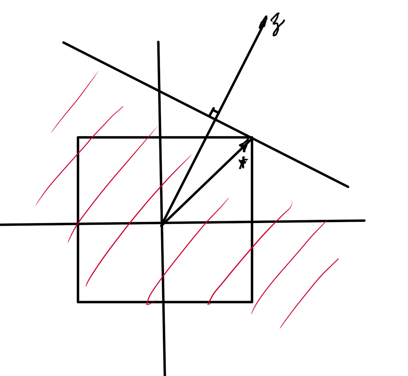
fig. 3. Half space containing the unit ball for l_infinity

and a similar pic for \( l_2 \), which is sketched in fig. 4.


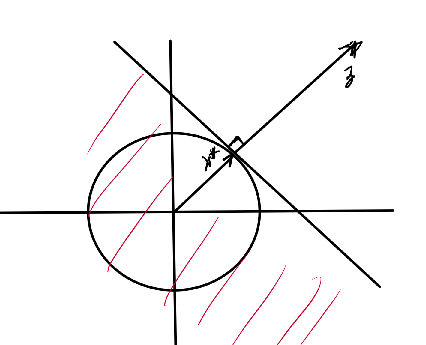
fig. 4. Half space containing for l_2 unit ball.

Q: What was this optimizer point?

Polyhedra

\begin{equation}\label{eqn:convexOptimizationLecture4:120}
\begin{aligned}
\mathcal{P}
&= \setlr{ \Bx |
\Ba_j^\T \Bx \le \Bb_j, j \in [1,m],
\Bc_i^\T \Bx = \Bd_i, i \in [1,p]
} \\
&=
\setlr{ \Bx | A \Bx \le \Bb, C \Bx = d },
\end{aligned}
\end{equation}

where the final inequality and equality are component wise.

Proving \( \mathcal{P} \) is convex:

  • Pick \(\Bx_1 \in \mathcal{P}\), \(\Bx_2 \in \mathcal{P} \)
  • Pick any \(\theta \in [0,1]\)
  • Test \( \theta \Bx_1 + (1-\theta) \Bx_2 \). Is it in \(\mathcal{P}\)?

\begin{equation}\label{eqn:convexOptimizationLecture4:140}
\begin{aligned}
A \lr{ \theta \Bx_1 + (1-\theta) \Bx_2 }
&=
\theta A \Bx_1 + (1-\theta) A \Bx_2 \\
&\le
\theta \Bb + (1-\theta) \Bb \\
&=
\Bb.
\end{aligned}
\end{equation}

Balls

Euclidean ball for \( \Bx_c \in \mathbb{R}^n, r \in \mathbb{R} \)

\begin{equation}\label{eqn:convexOptimizationLecture4:160}
\mathcal{B}(\Bx_c, r)
= \setlr{ \Bx | \Norm{\Bx – \Bx_c}_2 \le r },
\end{equation}

or
\begin{equation}\label{eqn:convexOptimizationLecture4:180}
\mathcal{B}(\Bx_c, r)
= \setlr{ \Bx | \lr{\Bx – \Bx_c}^\T \lr{\Bx – \Bx_c} \le r^2 }.
\end{equation}

Let \( \Bx_1, \Bx_2 \), \(\theta \in [0,1]\)

\begin{equation}\label{eqn:convexOptimizationLecture4:200}
\begin{aligned}
\Norm{ \theta \Bx_1 + (1-\theta) \Bx_2 – \Bx_c }_2
&=
\Norm{ \theta (\Bx_1 – \Bx_c) + (1-\theta) (\Bx_2 – \Bx_c) }_2 \\
&\le
\Norm{ \theta (\Bx_1 – \Bx_c)}_2 + \Norm{(1-\theta) (\Bx_2 – \Bx_c) }_2 \\
&=
\Abs{\theta} \Norm{ \Bx_1 – \Bx_c}_2 + \Abs{1 -\theta} \Norm{ \Bx_2 – \Bx_c }_2 \\
&=
\theta \Norm{ \Bx_1 – \Bx_c}_2 + \lr{1 -\theta} \Norm{ \Bx_2 – \Bx_c }_2 \\
&\le
\theta r + (1 – \theta) r \\
&= r
\end{aligned}
\end{equation}

Ellipse

\begin{equation}\label{eqn:convexOptimizationLecture4:220}
\mathcal{E}(\Bx_c, P)
=
\setlr{ \Bx | (\Bx – \Bx_c)^\T P^{-1} (\Bx – \Bx_c) \le 1 },
\end{equation}

where \( P \in S^n_{++} \).

  • Euclidean ball is an ellipse with \( P = I r^2 \)
  • Ellipse is image of Euclidean ball \( \mathcal{B}(0,1) \) under affine mapping.


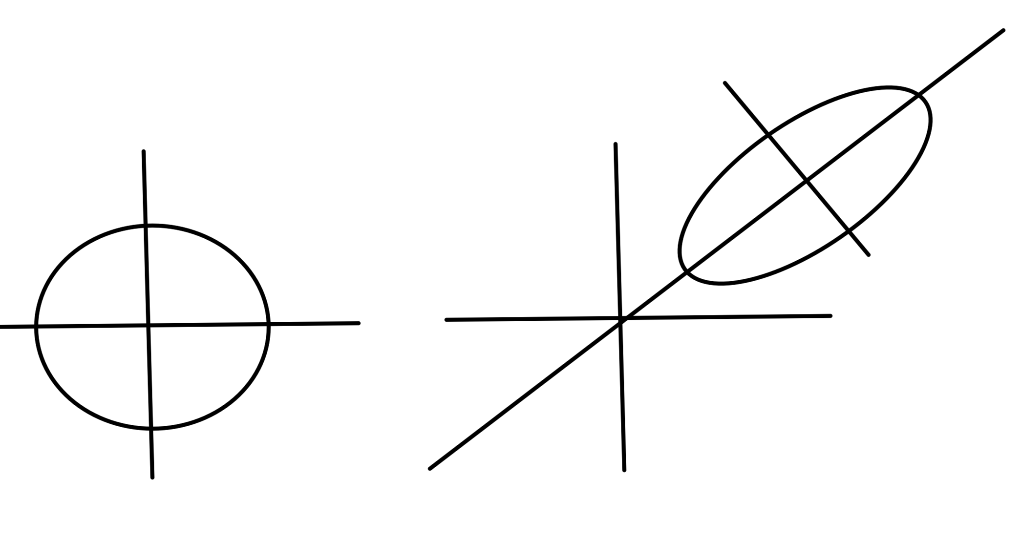
fig. 5. Circle and ellipse.

Given

\begin{equation}\label{eqn:convexOptimizationLecture4:240}
F(\Bu) = P^{1/2} \Bu + \Bx_c
\end{equation}

\begin{equation}\label{eqn:convexOptimizationLecture4:260}
\begin{aligned}
\setlr{ F(\Bu) | \Norm{\Bu}_2 \le r }
&=
\setlr{ P^{1/2} \Bu + \Bx_c | \Bu^\T \Bu \le r^2 } \\
&=
\setlr{ \Bx | \Bx = P^{1/2} \Bu + \Bx_c, \Bu^\T \Bu \le r^2 } \\
&=
\setlr{ \Bx | \Bu = P^{-1/2} (\Bx – \Bx_c), \Bu^\T \Bu \le r^2 } \\
&=
\setlr{ \Bx | (\Bx – \Bx_c)^\T P^{-1} (\Bx – \Bx_c) \le r^2 }
\end{aligned}
\end{equation}

Geometry of an ellipse

Decomposition of positive definite matrix \( P \in S^n_{++} \subset S^n \) is:

\begin{equation}\label{eqn:convexOptimizationLecture4:280}
\begin{aligned}
P &= Q \textrm{diag}(\lambda_i) Q^\T \\
Q^\T Q &= 1
\end{aligned},
\end{equation}

where \( \lambda_i \in \mathbb{R}\), and \(\lambda_i > 0 \). The ellipse is defined by

\begin{equation}\label{eqn:convexOptimizationLecture4:300}
(\Bx – \Bx_c)^\T Q \textrm{diag}(1/\lambda_i) (\Bx – \Bx_c) Q \le r^2
\end{equation}

The term \( (\Bx – \Bx_c)^\T Q \) projects \( \Bx – \Bx_c \) onto the columns of \( Q \). Those columns are perpendicular since \( Q \) is an orthogonal matrix. Let

\begin{equation}\label{eqn:convexOptimizationLecture4:320}
\tilde{\Bx} = Q^\T (\Bx – \Bx_c),
\end{equation}

this shifts the origin around \( \Bx_c \) and \( Q \) rotates into a new coordinate system. The ellipse is therefore

\begin{equation}\label{eqn:convexOptimizationLecture4:340}
\tilde{\Bx}^\T
\begin{bmatrix}
\inv{\lambda_1} & & & \\
&\inv{\lambda_2} & & \\
& \ddots & \\
& & & \inv{\lambda_n}
\end{bmatrix}
\tilde{\Bx}
=
\sum_{i = 1}^n \frac{\tilde{x}_i^2}{\lambda_i} \le 1.
\end{equation}

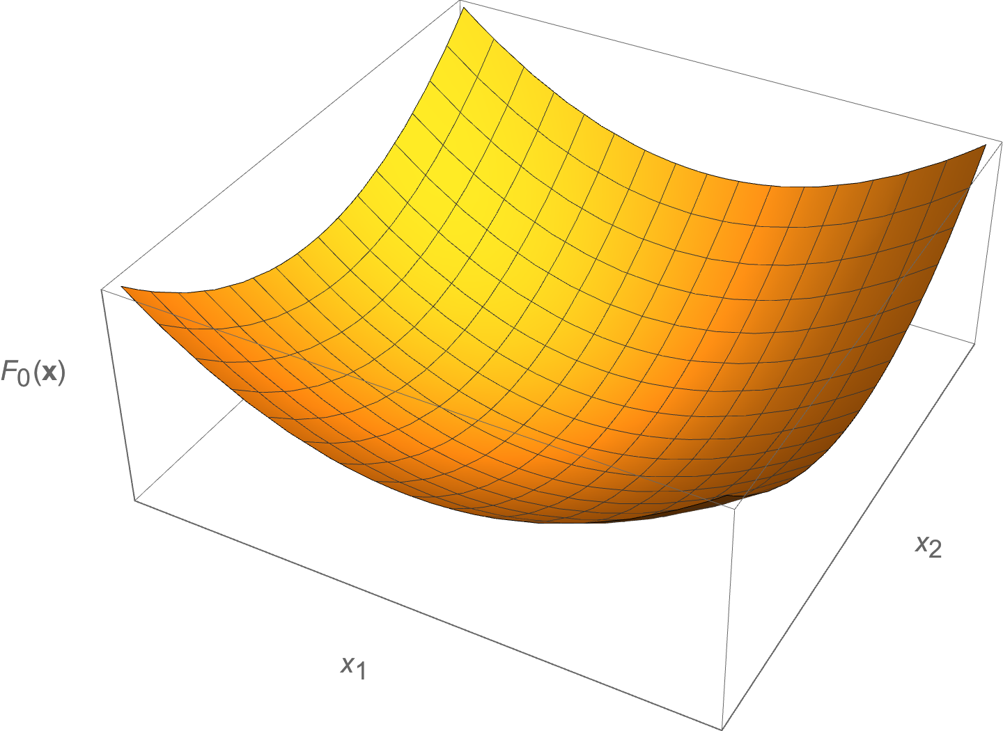
An example is sketched for \( \lambda_1 > \lambda_2 \) below.


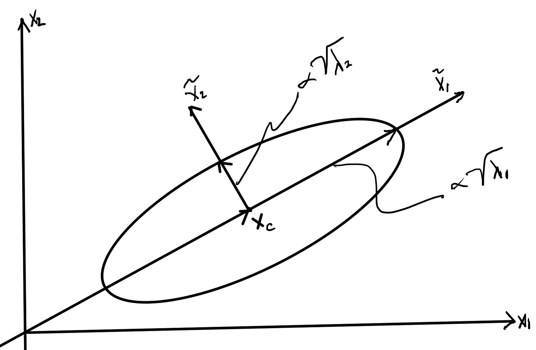
Ellipse with \( \lambda_1 > \lambda_2 \).

  • \( \lambda_i \) tells us length of the semi-major axis.
  • Larger \( \lambda_i \) means \( \tilde{x}_i^2 \) can be bigger and still satisfy constraint \( \le 1 \).
  • Volume of ellipse if proportional to \( \sqrt{ \det P } = \sqrt{ \prod_{i = 1}^n \lambda_i } \).
  • When any \( \lambda_i \rightarrow 0 \) a dimension is lost and the volume goes to zero. That removes the invertibility required.

Ellipses will be seen a lot in this course, since we are interested in “bowl” like geometries (and the ellipse is the image of a Euclidean ball).
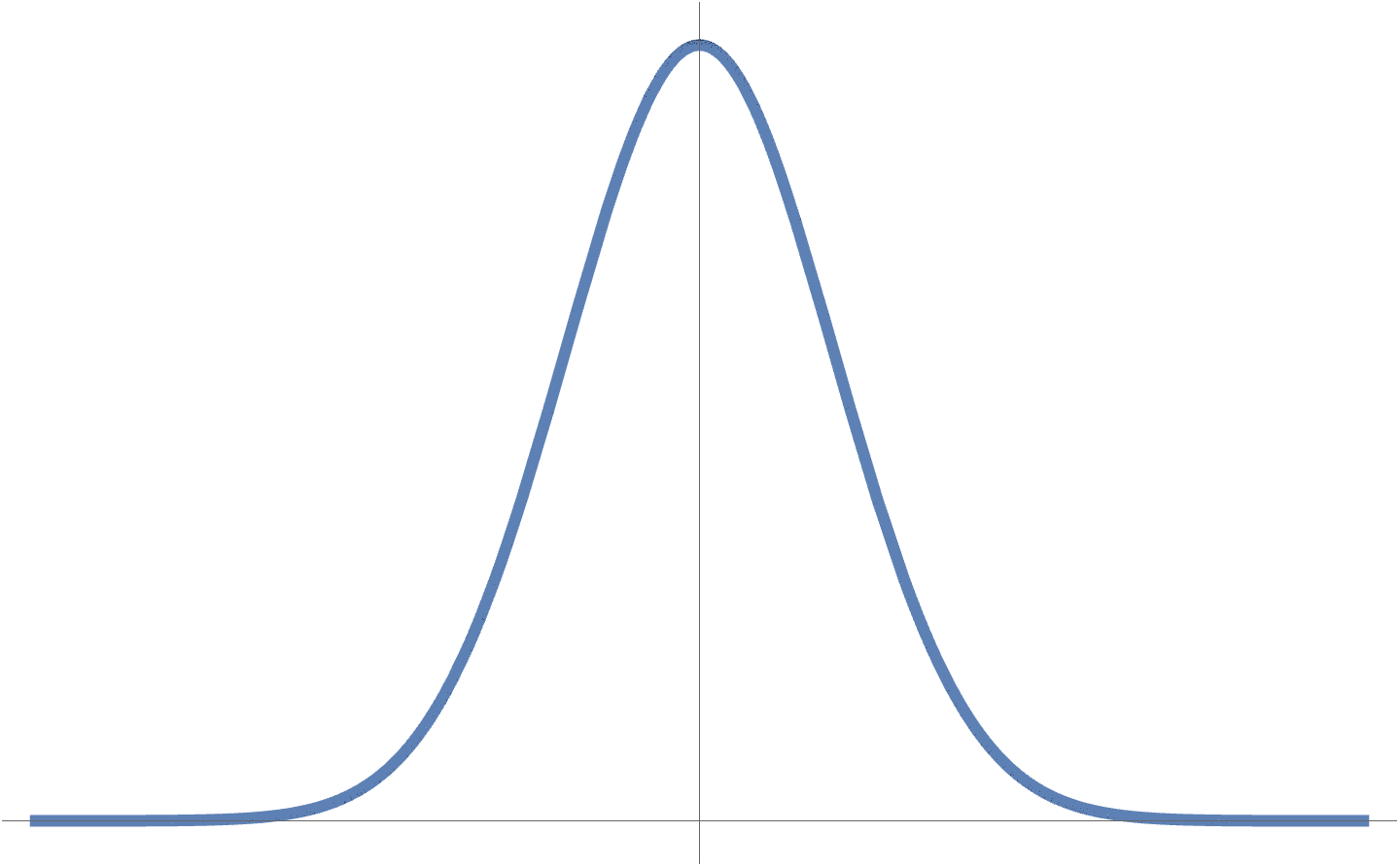
Norm ball.

The norm ball

\begin{equation}\label{eqn:convexOptimizationLecture4:360}
\mathcal{B} = \setlr{ \Bx | \Norm{\Bx} \le 1 },
\end{equation}

is a convex set for all norms. Proof:

Take any \( \Bx, \By \in \mathcal{B} \)

\begin{equation}\label{eqn:convexOptimizationLecture4:380}
\Norm{ \theta \Bx + (1 – \theta) \By }
\le
\Abs{\theta} \Norm{ \Bx } + \Abs{1 – \theta} \Norm{ \By }
=
\theta \Norm{ \Bx } + \lr{1 – \theta} \Norm{ \By }
\lr
\theta + \lr{1 – \theta}
=
1.
\end{equation}

This is true for any p-norm \( 1 \le p \), \( \Norm{\Bx}_p = \lr{ \sum_{i = 1}^n \Abs{x_i}^p }^{1/p} \).
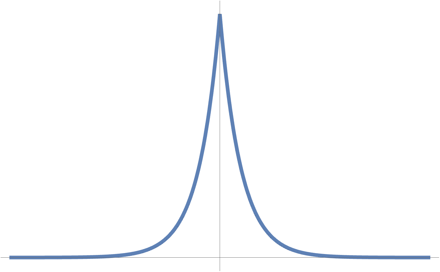
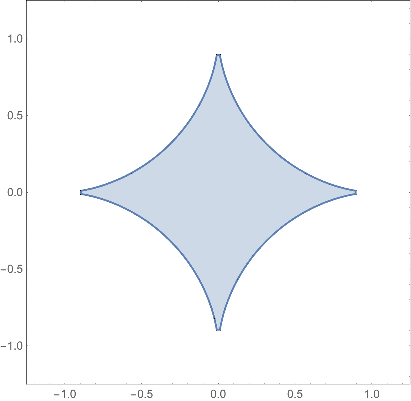
 

Norm ball.

The shape of a \( p < 1 \) norm unit ball is sketched below (lines connecting points in such a region can exit the region).
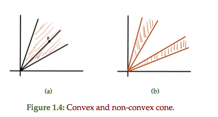
 

Cones

Recall that \( C \) is a cone if \( \forall \Bx \in C, \theta \ge 0, \theta \Bx \in C \).

Impt cone of PSD matrices

\begin{equation}\label{eqn:convexOptimizationLecture4:400}
\begin{aligned}
S^n &= \setlr{ X \in \mathbb{R}^{n \times n} | X = X^\T } \\
S^n_{+} &= \setlr{ X \in S^n | \Bv^\T X \Bv \ge 0, \quad \forall v \in \mathbb{R}^n } \\
S^n_{++} &= \setlr{ X \in S^n_{+} | \Bv^\T X \Bv > 0, \quad \forall v \in \mathbb{R}^n } \\
\end{aligned}
\end{equation}

These have respectively

  • \( \lambda_i \in \mathbb{R} \)
  • \( \lambda_i \in \mathbb{R}_{+} \)
  • \( \lambda_i \in \mathbb{R}_{++} \)

\( S^n_{+} \) is a cone if:

\( X \in S^n_{+}\), then \( \theta X \in S^n_{+}, \quad \forall \theta \ge 0 \)

\begin{equation}\label{eqn:convexOptimizationLecture4:420}
\Bv^\T (\theta X) \Bv
= \theta \Bv^\T \Bv
\ge 0,
\end{equation}

since \( \theta \ge 0 \) and because \( X \in S^n_{+} \).

Shorthand:

\begin{equation}\label{eqn:convexOptimizationLecture4:440}
\begin{aligned}
X &\in S^n_{+} \Rightarrow X \succeq 0
X &\in S^n_{++} \Rightarrow X \succ 0.
\end{aligned}
\end{equation}

Further \( S^n_{+} \) is a convex cone.

Let \( A \in S^n_{+} \), \( B \in S^n_{+} \), \( \theta_1, \theta_2 \ge 0, \theta_1 + \theta_2 = 1 \), or \( \theta_2 = 1 – \theta_1 \).

Show that \( \theta_1 A + \theta_2 B \in S^n_{+} \) :

\begin{equation}\label{eqn:convexOptimizationLecture4:460}
\Bv^\T \lr{ \theta_1 A + \theta_2 B } \Bv
=
\theta_1 \Bv^\T A \Bv
+\theta_2 \Bv^\T B \Bv
\ge 0,
\end{equation}

since \( \theta_1 \ge 0, \theta_2 \ge 0, \Bv^\T A \Bv \ge 0, \Bv^\T B \Bv \ge 0 \).
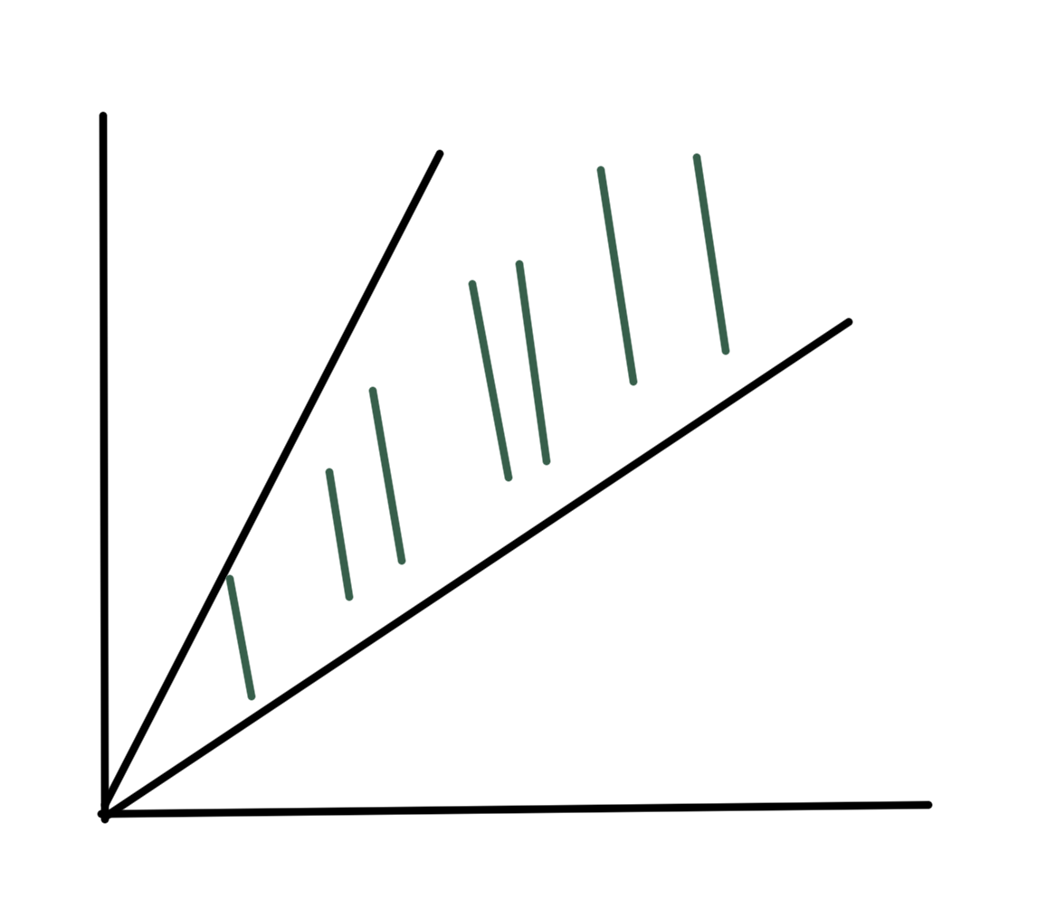
 

fig. 8. Cone.

Inequalities:

Start with a proper cone \( K \subseteq \mathbb{R}^n \)

  • closed, convex
  • non-empty interior (“solid”)
  • “pointed” (contains no lines)

The \( K \) defines a generalized inequality in \R{n} defined as “\(\le_K\)”

Interpreting

\begin{equation}\label{eqn:convexOptimizationLecture4:480}
\begin{aligned}
\Bx \le_K \By &\leftrightarrow \By – \Bx \in K
\Bx \end{aligned}
\end{equation}

Why pointed? Want if \( \Bx \le_K \By \) and \( \By \le_K \Bx \) with this \( K \) is a half space.

Example:1: \( K = \mathbb{R}^n_{+}, \Bx \in \mathbb{R}^n, \By \in \mathbb{R}^n \)


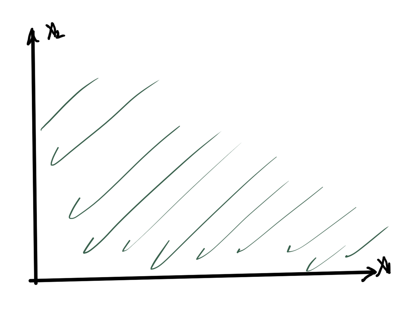
fig. 12. K is non-negative “orthant”

\begin{equation}\label{eqn:convexOptimizationLecture4:500}
\Bx \le_K \By \Rightarrow \By – \Bx \in K
\end{equation}

say:

\begin{equation}\label{eqn:convexOptimizationLecture4:520}
\begin{bmatrix}
y_1 – x_1
y_2 – x_2
\end{bmatrix}
\in R^2_{+}
\end{equation}

Also:

\begin{equation}\label{eqn:convexOptimizationLecture4:540}
K = R^1_{+}
\end{equation}

(pointed, since it contains no rays)

\begin{equation}\label{eqn:convexOptimizationLecture4:560}
\Bx \le_K \By ,
\end{equation}

with respect to \( K = \mathbb{R}^n_{+} \) means that \( x_i \le y_i \) for all \( i \in [1,n]\).

Example:2: For \( K = PSD \subseteq S^n \),

\begin{equation}\label{eqn:convexOptimizationLecture4:580}
\Bx \le_K \By ,
\end{equation}

means that

\begin{equation}\label{eqn:convexOptimizationLecture4:600}
\By – \Bx \in K = S^n_{+}.
\end{equation}

  • Difference \( \By – \Bx \) is always in \( S \)
  • check if in \( K \) by checking if all eigenvalues \( \ge 0 \).
  • \( S^n_{++} \) is the interior of \( S^n_{+} \).

Interpretation:

\begin{equation}\label{eqn:convexOptimizationLecture4:620}
\begin{aligned}
\Bx \le_K \By &\leftrightarrow \By – \Bx \in K \\
\Bx \end{aligned}
\end{equation}

We’ll use these with vectors and matrices so often the \( K \) subscript will often be dropped, writing instead (for vectors)

\begin{equation}\label{eqn:convexOptimizationLecture4:640}
\begin{aligned}
\Bx \le \By &\leftrightarrow \By – \Bx \in \mathbb{R}^n_{+} \\
\Bx < \By &\leftrightarrow \By – \Bx \in \textrm{int} \mathbb{R}^n_{++}
\end{aligned}
\end{equation}

and for matrices

\begin{equation}\label{eqn:convexOptimizationLecture4:660}
\begin{aligned}
\Bx \le \By &\leftrightarrow \By – \Bx \in S^n_{+} \\
\Bx < \By &\leftrightarrow \By – \Bx \in \textrm{int} S^n_{++}.
\end{aligned}
\end{equation}

Intersection

Take the intersection of (perhaps infinitely many) sets \( S_\alpha \):

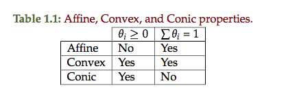
If \( S_\alpha \) is (affine,convex, conic) for all \( \alpha \in A \) then

\begin{equation}\label{eqn:convexOptimizationLecture4:680}
\cap_\alpha S_\alpha
\end{equation}

is (affine,convex, conic). To prove in homework:

\begin{equation}\label{eqn:convexOptimizationLecture4:700}
\mathcal{P} = \setlr{ \Bx | \Ba_i^\T \Bx \le \Bb_i, \Bc_j^\T \Bx = \Bd_j, \quad \forall i \cdots j }
\end{equation}

This is convex since the intersection of a bunch of hyperplane and half space constraints.

  1. If \( S \subseteq \mathbb{R}^n \) is convex then\begin{equation}\label{eqn:convexOptimizationLecture4:720}
    F(S) = \setlr{ F(\Bx) | \Bx \in S }
    \end{equation}is convex.
  2. If \( S \subseteq \mathbb{R}^m \) then\begin{equation}\label{eqn:convexOptimizationLecture4:740}
    F^{-1}(S) = \setlr{ \Bx | F(\Bx) \in S }
    \end{equation}is convex. Such a mapping is sketched in fig. 14.


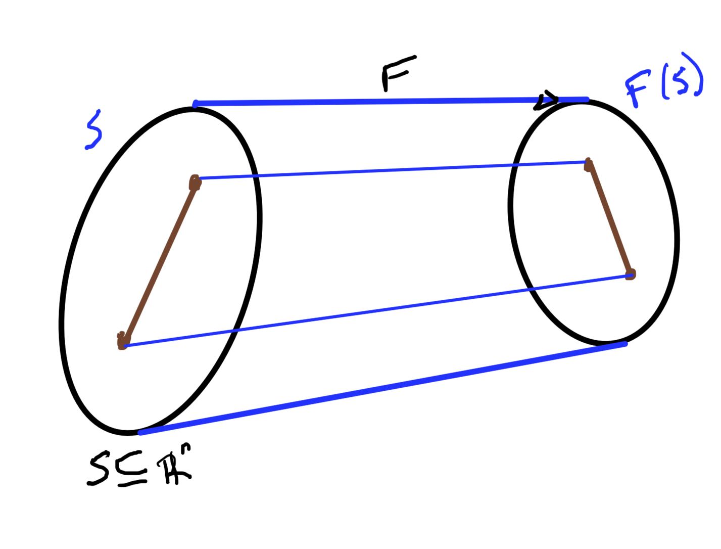
fig. 14. Mapping functions of sets.

References

[1] Stephen Boyd and Lieven Vandenberghe. Convex optimization. Cambridge university press, 2004.

ECE1505H Convex Optimization. Lecture 3: Matrix functions, SVD, and types of Sets. Taught by Prof. Stark Draper

January 19, 2017 ece1505 , , , , , , , , , , , , , , , , , , , ,

[Click here for a PDF of this post with nicer formatting]

Disclaimer

Peeter’s lecture notes from class. These may be incoherent and rough.

These are notes for the UofT course ECE1505H, Convex Optimization, taught by Prof. Stark Draper.

Matrix inner product

Given real matrices \( X, Y \in \mathbb{R}^{m\times n} \), one possible matrix inner product definition is

\begin{equation}\label{eqn:convexOptimizationLecture3:20}
\begin{aligned}
\innerprod{X}{Y}
&= \textrm{Tr}( X^\T Y) \\
&= \textrm{Tr} \lr{ \sum_{k = 1}^m X_{ki} Y_{kj} } \\
&= \sum_{k = 1}^m \sum_{j = 1}^n X_{kj} Y_{kj} \\
&= \sum_{i = 1}^m \sum_{j = 1}^n X_{ij} Y_{ij}.
\end{aligned}
\end{equation}

This inner product induces a norm on the (matrix) vector space, called the Frobenius norm

\begin{equation}\label{eqn:convexOptimizationLecture3:40}
\begin{aligned}
\Norm{X }_F
&= \textrm{Tr}( X^\T X) \\
&= \sqrt{ \innerprod{X}{X} } \\
&=
\sum_{i = 1}^m \sum_{j = 1}^n X_{ij}^2.
\end{aligned}
\end{equation}

Range, nullspace.

Definition: Range: Given \( A \in \mathbb{R}^{m \times n} \), the range of A is the set:

\begin{equation*}
\mathcal{R}(A) = \setlr{ A \Bx | \Bx \in \mathbb{R}^n }.
\end{equation*}

Definition: Nullspace: Given \( A \in \mathbb{R}^{m \times n} \), the nullspace of A is the set:

\begin{equation*}
\mathcal{N}(A) = \setlr{ \Bx | A \Bx = 0 }.
\end{equation*}

SVD.

To understand operation of \( A \in \mathbb{R}^{m \times n} \), a representation of a linear transformation from \R{n} to \R{m}, decompose \( A \) using the singular value decomposition (SVD).

Definition: SVD: Given \( A \in \mathbb{R}^{m \times n} \), an operator on \( \Bx \in \mathbb{R}^n \), a decomposition of the following form is always possible

\begin{equation*}
\begin{aligned}
A &= U \Sigma V^\T \\
U &\in \mathbb{R}^{m \times r} \\
V &\in \mathbb{R}^{n \times r},
\end{aligned}
\end{equation*}

where \( r \) is the rank of \(A\), and both \( U \) and \( V \) are orthogonal

\begin{equation*}
\begin{aligned}
U^\T U &= I \in \mathbb{R}^{r \times r} \\
V^\T V &= I \in \mathbb{R}^{r \times r}.
\end{aligned}
\end{equation*}

Here \( \Sigma = \textrm{diag}( \sigma_1, \sigma_2, \cdots, \sigma_r ) \), is a diagonal matrix of “singular” values, where

\begin{equation*}
\sigma_1 \ge \sigma_2 \ge \cdots \ge \sigma_r.
\end{equation*}

For simplicity consider square case \( m = n \)

\begin{equation}\label{eqn:convexOptimizationLecture3:100}
A \Bx = \lr{ U \Sigma V^\T } \Bx.
\end{equation}

The first product \( V^\T \Bx \) is a rotation, which can be checked by looking at the length

\begin{equation}\label{eqn:convexOptimizationLecture3:120}
\begin{aligned}
\Norm{ V^\T \Bx}_2
&= \sqrt{ \Bx^\T V V^\T \Bx } \\
&= \sqrt{ \Bx^\T \Bx } \\
&= \Norm{ \Bx }_2,
\end{aligned}
\end{equation}

which shows that the length of the vector is unchanged after application of the linear transformation represented by \( V^\T \) so that operation must be a rotation.

Similarly the operation of \( U \) on \( \Sigma V^\T \Bx \) also must be a rotation. The operation \( \Sigma = [\sigma_i]_i \) applies a scaling operation to each component of the vector \( V^\T \Bx \).

All linear (square) transformations can therefore be thought of as a rotate-scale-rotate operation. Often the \( A \) of interest will be symmetric \( A = A^\T \).

Set of symmetric matrices

Let \( S^n \) be the set of real, symmetric \( n \times n \) matrices.

Theorem: Spectral theorem: When \( A \in S^n \) then it is possible to factor \( A \) as

\begin{equation*}
A = Q \Lambda Q^\T,
\end{equation*}

where \( Q \) is an orthogonal matrix, and \( \Lambda = \textrm{diag}( \lambda_1, \lambda_2, \cdots \lambda_n)\). Here \( \lambda_i \in \mathbb{R} \, \forall i \) are the (real) eigenvalues of \( A \).

A real symmetric matrix \( A \in S^n\) is “positive semi-definite” if

\begin{equation*}
\Bv^\T A \Bv \ge 0 \qquad\forall \Bv \in \mathbb{R}^n, \Bv \ne 0,
\end{equation*}
and is “positive definite” if

\begin{equation*}
\Bv^\T A \Bv > 0 \qquad\forall \Bv \in \mathbb{R}^n, \Bv \ne 0.
\end{equation*}

The set of such matrices is denoted \( S^n_{+} \), and \( S^n_{++} \) respectively.

Consider \( A \in S^n_{+} \) (or \( S^n_{++} \) )

\begin{equation}\label{eqn:convexOptimizationLecture3:200}
A = Q \Lambda Q^\T,
\end{equation}

possible since the matrix is symmetric. For such a matrix

\begin{equation}\label{eqn:convexOptimizationLecture3:220}
\begin{aligned}
\Bv^\T A \Bv
&=
\Bv^\T Q \Lambda A^\T \Bv \\
&=
\Bw^\T \Lambda \Bw,
\end{aligned}
\end{equation}

where \( \Bw = A^\T \Bv \). Such a product is

\begin{equation}\label{eqn:convexOptimizationLecture3:240}
\Bv^\T A \Bv
=
\sum_{i = 1}^n \lambda_i w_i^2.
\end{equation}

So, if \( \lambda_i \ge 0 \) (\(\lambda_i > 0 \) ) then \( \sum_{i = 1}^n \lambda_i w_i^2 \) is non-negative (positive) \( \forall \Bw \in \mathbb{R}^n, \Bw \ne 0 \). Since \( \Bw \) is just a rotated version of \( \Bv \) this also holds for all \( \Bv \). A necessary and sufficient condition for \( A \in S^n_{+} \) (\( S^n_{++} \) ) is \( \lambda_i \ge 0 \) (\(\lambda_i > 0\)).

Square root of positive semi-definite matrix

Real symmetric matrix power relationships such as

\begin{equation}\label{eqn:convexOptimizationLecture3:260}
A^2
=
Q \Lambda Q^\T
Q \Lambda Q^\T
=
Q \Lambda^2
Q^\T
,
\end{equation}

or more generally \( A^k = Q \Lambda^k Q^\T,\, k \in \mathbb{Z} \), can be further generalized to non-integral powers. In particular, the square root (non-unique) of a square matrix can be written

\begin{equation}\label{eqn:convexOptimizationLecture3:280}
A^{1/2} = Q
\begin{bmatrix}
\sqrt{\lambda_1} & & & \\
& \sqrt{\lambda_2} & & \\
& & \ddots & \\
& & & \sqrt{\lambda_n} \\
\end{bmatrix}
Q^\T,
\end{equation}

since \( A^{1/2} A^{1/2} = A \), regardless of the sign picked for the square roots in question.

Functions of matrices

Consider \( F : S^n \rightarrow \mathbb{R} \), and define

\begin{equation}\label{eqn:convexOptimizationLecture3:300}
F(X) = \log \det X,
\end{equation}

Here \( \textrm{dom} F = S^n_{++} \). The task is to find \( \spacegrad F \), which can be done by looking at the perturbation \( \log \det ( X + \Delta X ) \)

\begin{equation}\label{eqn:convexOptimizationLecture3:320}
\begin{aligned}
\log \det ( X + \Delta X )
&=
\log \det ( X^{1/2} (I + X^{-1/2} \Delta X X^{-1/2}) X^{1/2} ) \\
&=
\log \det ( X (I + X^{-1/2} \Delta X X^{-1/2}) ) \\
&=
\log \det X + \log \det (I + X^{-1/2} \Delta X X^{-1/2}).
\end{aligned}
\end{equation}

Let \( X^{-1/2} \Delta X X^{-1/2} = M \) where \( \lambda_i \) are the eigenvalues of \( M : M \Bv = \lambda_i \Bv \) when \( \Bv \) is an eigenvector of \( M \). In particular

\begin{equation}\label{eqn:convexOptimizationLecture3:340}
(I + M) \Bv =
(1 + \lambda_i) \Bv,
\end{equation}

where \( 1 + \lambda_i \) are the eigenvalues of the \( I + M \) matrix. Since the determinant is the product of the eigenvalues, this gives

\begin{equation}\label{eqn:convexOptimizationLecture3:360}
\begin{aligned}
\log \det ( X + \Delta X )
&=
\log \det X +
\log \prod_{i = 1}^n (1 + \lambda_i) \\
&=
\log \det X +
\sum_{i = 1}^n \log (1 + \lambda_i).
\end{aligned}
\end{equation}

If \( \lambda_i \) are sufficiently “small”, then \( \log ( 1 + \lambda_i ) \approx \lambda_i \), giving

\begin{equation}\label{eqn:convexOptimizationLecture3:380}
\log \det ( X + \Delta X )
=
\log \det X +
\sum_{i = 1}^n \lambda_i
\approx
\log \det X +
\textrm{Tr}( X^{-1/2} \Delta X X^{-1/2} ).
\end{equation}

Since
\begin{equation}\label{eqn:convexOptimizationLecture3:400}
\textrm{Tr}( A B ) = \textrm{Tr}( B A ),
\end{equation}

this trace operation can be written as

\begin{equation}\label{eqn:convexOptimizationLecture3:420}
\log \det ( X + \Delta X )
\approx
\log \det X +
\textrm{Tr}( X^{-1} \Delta X )
=
\log \det X +
\innerprod{ X^{-1}}{\Delta X},
\end{equation}

so
\begin{equation}\label{eqn:convexOptimizationLecture3:440}
\spacegrad F(X) = X^{-1}.
\end{equation}

To check this, consider the simplest example with \( X \in \mathbb{R}^{1 \times 1} \), where we have

\begin{equation}\label{eqn:convexOptimizationLecture3:460}
\frac{d}{dX} \lr{ \log \det X } = \frac{d}{dX} \lr{ \log X } = \inv{X} = X^{-1}.
\end{equation}

This is a nice example demonstrating how the gradient can be obtained by performing a first order perturbation of the function. The gradient can then be read off from the result.

Second order perturbations

  • To get first order approximation found the part that varied linearly in \( \Delta X \).
  • To get the second order part, perturb \( X^{-1} \) by \( \Delta X \) and see how that perturbation varies in \( \Delta X \).

For \( G(X) = X^{-1} \), this is

\begin{equation}\label{eqn:convexOptimizationLecture3:480}
\begin{aligned}
(X + \Delta X)^{-1}
&=
\lr{ X^{1/2} (I + X^{-1/2} \Delta X X^{-1/2} ) X^{1/2} }^{-1} \\
&=
X^{-1/2} (I + X^{-1/2} \Delta X X^{-1/2} )^{-1} X^{-1/2}
\end{aligned}
\end{equation}

To be proven in the homework (for “small” A)

\begin{equation}\label{eqn:convexOptimizationLecture3:500}
(I + A)^{-1} \approx I – A.
\end{equation}

This gives

\begin{equation}\label{eqn:convexOptimizationLecture3:520}
\begin{aligned}
(X + \Delta X)^{-1}
&=
X^{-1/2} (I – X^{-1/2} \Delta X X^{-1/2} ) X^{-1/2} \\
&=
X^{-1} – X^{-1} \Delta X X^{-1},
\end{aligned}
\end{equation}

or

\begin{equation}\label{eqn:convexOptimizationLecture3:800}
\begin{aligned}
G(X + \Delta X)
&= G(X) + (D G) \Delta X \\
&= G(X) + (\spacegrad G)^\T \Delta X,
\end{aligned}
\end{equation}

so
\begin{equation}\label{eqn:convexOptimizationLecture3:820}
(\spacegrad G)^\T \Delta X
=
– X^{-1} \Delta X X^{-1}.
\end{equation}

The Taylor expansion of \( F \) to second order is

\begin{equation}\label{eqn:convexOptimizationLecture3:840}
F(X + \Delta X)
=
F(X)
+
\textrm{Tr} \lr{ (\spacegrad F)^\T \Delta X}
+
\inv{2}
\lr{ (\Delta X)^\T (\spacegrad^2 F) \Delta X}.
\end{equation}

The first trace can be expressed as an inner product

\begin{equation}\label{eqn:convexOptimizationLecture3:860}
\begin{aligned}
\textrm{Tr} \lr{ (\spacegrad F)^\T \Delta X}
&=
\innerprod{ \spacegrad F }{\Delta X} \\
&=
\innerprod{ X^{-1} }{\Delta X}.
\end{aligned}
\end{equation}

The second trace also has the structure of an inner product

\begin{equation}\label{eqn:convexOptimizationLecture3:880}
\begin{aligned}
(\Delta X)^\T (\spacegrad^2 F) \Delta X
&=
\textrm{Tr} \lr{ (\Delta X)^\T (\spacegrad^2 F) \Delta X} \\
&=
\innerprod{ (\spacegrad^2 F)^\T \Delta X }{\Delta X},
\end{aligned}
\end{equation}

where a no-op trace could be inserted in the second order term since that quadratic form is already a scalar. This \( (\spacegrad^2 F)^\T \Delta X \) term has essentially been found implicitly by performing the linear variation of \( \spacegrad F \) in \( \Delta X \), showing that we must have

\begin{equation}\label{eqn:convexOptimizationLecture3:900}
\textrm{Tr} \lr{ (\Delta X)^\T (\spacegrad^2 F) \Delta X}
=
\innerprod{ – X^{-1} \Delta X X^{-1} }{\Delta X},
\end{equation}

so
\begin{equation}\label{eqn:convexOptimizationLecture3:560}
F( X + \Delta X) = F(X) +
\innerprod{X^{-1}}{\Delta X}
+\inv{2} \innerprod{-X^{-1} \Delta X X^{-1}}{\Delta X},
\end{equation}

or
\begin{equation}\label{eqn:convexOptimizationLecture3:580}
\log \det ( X + \Delta X) = \log \det X +
\textrm{Tr}( X^{-1} \Delta X )
– \inv{2} \textrm{Tr}( X^{-1} \Delta X X^{-1} \Delta X ).
\end{equation}

Convex Sets

  • Types of sets: Affine, convex, cones
  • Examples: Hyperplanes, polyhedra, balls, ellipses, norm balls, cone of PSD matrices.

Definition: Affine set:

A set \( C \subseteq \mathbb{R}^n \) is affine if \( \forall \Bx_1, \Bx_2 \in C \) then

\begin{equation*}
\theta \Bx_1 + (1 -\theta) \Bx_2 \in C, \qquad \forall \theta \in \mathbb{R}.
\end{equation*}

The affine sum above can
be rewritten as

\begin{equation}\label{eqn:convexOptimizationLecture3:600}
\Bx_2 + \theta (\Bx_1 – \Bx_2).
\end{equation}

Since \( \theta \) is a scaling, this is the line containing \( \Bx_2 \) in the direction between \( \Bx_1 \) and \( \Bx_2 \).

Observe that the solution to a set of linear equations

\begin{equation}\label{eqn:convexOptimizationLecture3:620}
C = \setlr{ \Bx | A \Bx = \Bb },
\end{equation}

is an affine set. To check, note that

\begin{equation}\label{eqn:convexOptimizationLecture3:640}
\begin{aligned}
A (\theta \Bx_1 + (1 – \theta) \Bx_2)
&=
\theta A \Bx_1 + (1 – \theta) A \Bx_2 \\
&=
\theta \Bb + (1 – \theta) \Bb \\
&= \Bb.
\end{aligned}
\end{equation}

Definition: Affine combination: An affine combination of points \( \Bx_1, \Bx_2, \cdots \Bx_n \) is

\begin{equation*}
\sum_{i = 1}^n \theta_i \Bx_i,
\end{equation*}

such that for \( \theta_i \in \mathbb{R} \)

\begin{equation*}
\sum_{i = 1}^n \theta_i = 1.
\end{equation*}

An affine set contains all affine combinations of points in the set. Examples of a couple affine sets are sketched in fig 1.1

For comparison, a couple of non-affine sets are sketched in fig 1.2


Definition: Convex set: A set \( C \subseteq \mathbb{R}^n \) is convex if \( \forall \Bx_1, \Bx_2 \in C \) and \( \forall \theta \in \mathbb{R}, \theta \in [0,1] \), the combination

\begin{equation}\label{eqn:convexOptimizationLecture3:700}
\theta \Bx_1 + (1 – \theta) \Bx_2 \in C.
\end{equation}

Definition: Convex combination: A convex combination of \( \Bx_1, \Bx_2, \cdots \Bx_n \) is

\begin{equation*}
\sum_{i = 1}^n \theta_i \Bx_i,
\end{equation*}

such that \( \forall \theta_i \ge 0 \)

\begin{equation*}
\sum_{i = 1}^n \theta_i = 1
\end{equation*}

Definition: Convex hull: Convex hull of a set \( C \) is a set of all convex combinations of points in \(C\), denoted

\begin{equation}\label{eqn:convexOptimizationLecture3:720}
\textrm{conv}(C) = \setlr{ \sum_{i=1}^n \theta_i \Bx_i | \Bx_i \in C, \theta_i \ge 0, \sum_{i=1}^n \theta_i = 1 }.
\end{equation}

A non-convex set can be converted into a convex hull by filling in all the combinations of points connecting points in the set, as sketched in fig 1.3.

Definition: Cone: A set \(C\) is a cone if \( \forall \Bx \in C \) and \( \forall \theta \ge 0 \) we have \( \theta \Bx \in C\).

This scales out if \(\theta > 1\) and scales in if \(\theta < 1\).

A convex cone is a cone that is also a convex set. A conic combination is

\begin{equation*}
\sum_{i=1}^n \theta_i \Bx_i, \theta_i \ge 0.
\end{equation*}

A convex and non-convex 2D cone is sketched in fig. 1.4

A comparison of properties for different set types is tabulated in table 1.1

Hyperplanes and half spaces

Definition: Hyperplane: A hyperplane is defined by

\begin{equation*}
\setlr{ \Bx | \Ba^\T \Bx = \Bb, \Ba \ne 0 }.
\end{equation*}

A line and plane are examples of this general construct as sketched in
fig. 1.5

An alternate view is possible should one
find any specific \( \Bx_0 \) such that \( \Ba^\T \Bx_0 = \Bb \)

\begin{equation}\label{eqn:convexOptimizationLecture3:740}
\setlr{\Bx | \Ba^\T \Bx = b }
=
\setlr{\Bx | \Ba^\T (\Bx -\Bx_0) = 0 }
\end{equation}

This shows that \( \Bx – \Bx_0 = \Ba^\perp \) is perpendicular to \( \Ba \), or

\begin{equation}\label{eqn:convexOptimizationLecture3:780}
\Bx
=
\Bx_0 + \Ba^\perp.
\end{equation}

This is the subspace perpendicular to \( \Ba \) shifted by \(\Bx_0\), subject to \( \Ba^\T \Bx_0 = \Bb \). As a set

\begin{equation}\label{eqn:convexOptimizationLecture3:760}
\Ba^\perp = \setlr{ \Bv | \Ba^\T \Bv = 0 }.
\end{equation}

Half space

Definition: Half space: The half space is defined as
\begin{equation*}
\setlr{ \Bx | \Ba^\T \Bx = \Bb }
= \setlr{ \Bx | \Ba^\T (\Bx – \Bx_0) \le 0 }.
\end{equation*}

This can also be expressed as \( \setlr{ \Bx | \innerprod{ \Ba }{\Bx – \Bx_0 } \le 0 } \).

ECE1505H Convex Optimization. Lecture 2: Mathematical background. Taught by Prof. Stark Draper

January 17, 2017 ece1505 , , , , , , , ,

[Click here for a PDF of this post with nicer formatting]

Disclaimer

Peeter’s lecture notes from class. These may be incoherent and rough.

These are notes for the UofT course ECE1505H, Convex Optimization, taught by Prof. Stark Draper, from [1].

Topics

  • Calculus: Derivatives and Jacobians, Gradients, Hessians, approximation functions.
  • Linear algebra, Matrices, decompositions, …

Norms

Vector space:

A set of elements (vectors) that is closed under vector addition and scaling.

This generalizes the directed arrow concept of vector space (fig. 1) that is familiar from geometry.

fig. 1. Vector addition.

Normed vector spaces:

A vector space with a notion of length of any single vector, the “norm”.

Inner product space:
A normed vector space with a notion of a real angle between any pair of vectors.

This course has a focus on optimization in \R{n}. Complex spaces in the context of this course can be considered with a mapping \( \text{\C{n}} \rightarrow \mathbb{R}^{2 n} \).

Norm:
A norm is a function operating on a vector

\begin{equation*}
\Bx = ( x_1, x_2, \cdots, x_n )
\end{equation*}

that provides a mapping

\begin{equation*}
\Norm{ \cdot } : \mathbb{R}^{n} \rightarrow \mathbb{R},
\end{equation*}

where

  • \( \Norm{ \Bx } \ge 0 \)
  • \( \Norm{ \Bx } = 0 \qquad \iff \Bx = 0 \)
  • \( \Norm{ t \Bx } = \Abs{t} \Norm{ \Bx } \)
  • \( \Norm{ \Bx + \By } \le \Norm{ \Bx } + \Norm{\By} \). This is the triangle inequality.

Example: Euclidean norm

\begin{equation}\label{eqn:convex-optimizationLecture2:24}
\Norm{\Bx} = \sqrt{ \sum_{i = 1}^n x_i^2 }
\end{equation}

Example: \(l_p\)-norms

\begin{equation}\label{eqn:convex-optimizationLecture2:44}
\Norm{\Bx}_p = \lr{ \sum_{i = 1}^n \Abs{x_i}^p }^{1/p}.
\end{equation}

For \( p = 1 \), this is

\begin{equation}\label{eqn:convex-optimizationLecture2:64}
\Norm{\Bx}_1 = \sum_{i = 1}^n \Abs{x_i},
\end{equation}

For \( p = 2 \), this is the Euclidean norm \ref{eqn:convex-optimizationLecture2:24}.
For \( p = \infty \), this is

\begin{equation}\label{eqn:convex-optimizationLecture2:324}
\Norm{\Bx}_\infty = \max_{i = 1}^n \Abs{x_i}.
\end{equation}

Unit ball:

\begin{equation*}
\setlr{ \Bx | \Norm{\Bx} \le 1 }
\end{equation*}

The regions of the unit ball under the \( l_1, l_2, and l_\infty \) norms are plotted in fig. 2.

fig. 2. Some unit ball regions.

The \( l_2 \) norm is not only familiar, but can be “induced” by an inner product

\begin{equation}\label{eqn:convex-optimizationLecture2:84}
\left\langle \Bx, \By \right\rangle = \Bx^\T \By = \sum_{i = 1}^n x_i y_i,
\end{equation}

which is not true for all norms. The norm induced by this inner product is

\begin{equation}\label{eqn:convex-optimizationLecture2:104}
\Norm{\Bx}_2 = \sqrt{ \left\langle \Bx, \By \right\rangle }
\end{equation}

Inner product spaces have a notion of angle (fig. 3) given by

\begin{equation}\label{eqn:convex-optimizationLecture2:124}
\left\langle \Bx, \By \right\rangle = \Norm{\Bx} \Norm{\By} \cos \theta,
\end{equation}


fig. 3. Inner product induced angle.

and always satisfy the Cauchy-Schwartz inequality

\begin{equation}\label{eqn:convex-optimizationLecture2:144}
\left\langle \Bx, \By \right\rangle \le \Norm{\Bx}_2 \Norm{\By}_2.
\end{equation}

In an inner product space we say \( \Bx \) and \( \By \) are orthogonal vectors \( \Bx \perp \By \) if \( \left\langle \Bx, \By \right\rangle = 0 \), as sketched in fig. 4.


fig. 4. Orthogonality.

Dual norm

Let \( \Norm{ \cdot } \) be a norm in \R{n}. The “dual” norm \( \Norm{ \cdot }_\conj \) is defined as

\begin{equation*}
\Norm{\Bz}_\conj = \sup_\Bx \setlr{ \Bz^\T \Bx | \Norm{\Bx} \le 1 }.
\end{equation*}

where \( \sup \) is roughly the “least upper bound”.
\index{sup}

This is a limit over the unit ball of \( \Norm{\cdot} \).

\( l_2 \) dual

Dual of the \( l_2 \) is the \( l_2 \) norm.

fig. 5. l_2 dual norm determination.


Proof:

\begin{equation}\label{eqn:convex-optimizationLecture2:164}
\begin{aligned}
\Norm{\Bz}_\conj
&= \sup_\Bx \setlr{ \Bz^\T \Bx | \Norm{\Bx}_2 \le 1 } \\
&= \sup_\Bx \setlr{ \Norm{\Bz}_2 \Norm{\Bx}_2 \cos\theta | \Norm{\Bx}_2 \le 1 } \\
&\le \sup_\Bx \setlr{ \Norm{\Bz}_2 \Norm{\Bx}_2 | \Norm{\Bx}_2 \le 1 } \\
&\le
\Norm{\Bz}_2
\Norm{
\frac{\Bz}{ \Norm{\Bz}_2 }
}_2 \\
&=
\Norm{\Bz}_2.
\end{aligned}
\end{equation}

\( l_1 \) dual

For \( l_1 \), the dual is the \( l_\infty \) norm. Proof:

\begin{equation}\label{eqn:convex-optimizationLecture2:184}
\Norm{\Bz}_\conj
=
\sup_\Bx \setlr{ \Bz^\T \Bx | \Norm{\Bx}_1 \le 1 },
\end{equation}

but
\begin{equation}\label{eqn:convex-optimizationLecture2:204}
\Bz^\T \Bx
=
\sum_{i=1}^n z_i x_i \le
\Abs{
\sum_{i=1}^n z_i x_i
}
\le
\sum_{i=1}^n \Abs{z_i x_i },
\end{equation}

so
\begin{equation}\label{eqn:convex-optimizationLecture2:224}
\begin{aligned}
\Norm{\Bz}_\conj
&=
\sum_{i=1}^n \Abs{z_i}\Abs{ x_i } \\
&\le \lr{ \max_{j=1}^n \Abs{z_j} }
\sum_{i=1}^n \Abs{ x_i } \\
&\le \lr{ \max_{j=1}^n \Abs{z_j} } \\
&=
\Norm{\Bz}_\infty.
\end{aligned}
\end{equation}


\( l_\infty \) dual

.

fig. 6. l_1 dual norm determination.

fig. 7. l_\infinity dual norm determination.

\begin{equation}\label{eqn:convex-optimizationLecture2:244}
\Norm{\Bz}_\conj
=
\sup_\Bx \setlr{ \Bz^\T \Bx | \Norm{\Bx}_\infty \le 1 }.
\end{equation}

Here
\begin{equation}\label{eqn:convex-optimizationLecture2:264}
\begin{aligned}
\Bz^\T \Bx
&=
\sum_{i=1}^n z_i x_i \\
&\le
\sum_{i=1}^n \Abs{z_i}\Abs{ x_i } \\
&\le
\lr{ \max_j \Abs{ x_j } }
\sum_{i=1}^n \Abs{z_i} \\
&=
\Norm{\Bx}_\infty
\sum_{i=1}^n \Abs{z_i}.
\end{aligned}
\end{equation}

So
\begin{equation}\label{eqn:convex-optimizationLecture2:284}
\Norm{\Bz}_\conj
\le
\sum_{i=1}^n \Abs{z_i}
=
\Norm{\Bz}_1.
\end{equation}

Statement from the lecture: I’m not sure where this fits:

\begin{equation}\label{eqn:convex-optimizationLecture2:304}
x_i^\conj
=
\left\{
\begin{array}{l l}
+1 & \quad \mbox{\( z_i \ge 0 \)} \\
-1 & \quad \mbox{\( z_i \le 0 \)}
\end{array}
\right.
\end{equation}

References

[1] Stephen Boyd and Lieven Vandenberghe. Convex optimization. Cambridge university press, 2004.

Jacobian and Hessian matrices

January 15, 2017 ece1505 , , , , , ,

[Click here for a PDF of this post with nicer formatting]

Motivation

In class this Friday the Jacobian and Hessian matrices were introduced, but I did not find the treatment terribly clear. Here is an alternate treatment, beginning with the gradient construction from [2], which uses a nice trick to frame the multivariable derivative operation as a single variable Taylor expansion.

Multivariable Taylor approximation

The Taylor series expansion for a scalar function \( g : {\mathbb{R}} \rightarrow {\mathbb{R}} \) about the origin is just

\begin{equation}\label{eqn:jacobianAndHessian:20}
g(t) = g(0) + t g'(0) + \frac{t^2}{2} g”(0) + \cdots
\end{equation}

In particular

\begin{equation}\label{eqn:jacobianAndHessian:40}
g(1) = g(0) + g'(0) + \frac{1}{2} g”(0) + \cdots
\end{equation}

Now consider \( g(t) = f( \Bx + \Ba t ) \), where \( f : {\mathbb{R}}^n \rightarrow {\mathbb{R}} \), \( g(0) = f(\Bx) \), and \( g(1) = f(\Bx + \Ba) \). The multivariable Taylor expansion now follows directly

\begin{equation}\label{eqn:jacobianAndHessian:60}
f( \Bx + \Ba)
= f(\Bx)
+ \evalbar{\frac{df(\Bx + \Ba t)}{dt}}{t = 0} + \frac{1}{2} \evalbar{\frac{d^2f(\Bx + \Ba t)}{dt^2}}{t = 0} + \cdots
\end{equation}

The first order term is

\begin{equation}\label{eqn:jacobianAndHessian:80}
\begin{aligned}
\evalbar{\frac{df(\Bx + \Ba t)}{dt}}{t = 0}
&=
\sum_{i = 1}^n
\frac{d( x_i + a_i t)}{dt}
\evalbar{\PD{(x_i + a_i t)}{f(\Bx + \Ba t)}}{t = 0} \\
&=
\sum_{i = 1}^n
a_i
\PD{x_i}{f(\Bx)} \\
&= \Ba \cdot \spacegrad f.
\end{aligned}
\end{equation}

Similarily, for the second order term

\begin{equation}\label{eqn:jacobianAndHessian:100}
\begin{aligned}
\evalbar{\frac{d^2 f(\Bx + \Ba t)}{dt^2}}{t = 0}
&=
\evalbar{\lr{
\frac{d}{dt}
\lr{
\sum_{i = 1}^n
a_i
\PD{(x_i + a_i t)}{f(\Bx + \Ba t)}
}
}
}{t = 0} \\
&=
\evalbar{
\lr{
\sum_{j = 1}^n
\frac{d(x_j + a_j t)}{dt}
\sum_{i = 1}^n
a_i
\frac{\partial^2 f(\Bx + \Ba t)}{\partial (x_j + a_j t) \partial (x_i + a_i t) }
}
}{t = 0} \\
&=
\sum_{i,j = 1}^n a_i a_j \frac{\partial^2 f}{\partial x_i \partial x_j} \\
&=
(\Ba \cdot \spacegrad)^2 f.
\end{aligned}
\end{equation}

The complete Taylor expansion of a scalar function \( f : {\mathbb{R}}^n \rightarrow {\mathbb{R}} \) is therefore

\begin{equation}\label{eqn:jacobianAndHessian:120}
f(\Bx + \Ba)
= f(\Bx) +
\Ba \cdot \spacegrad f +
\inv{2} \lr{ \Ba \cdot \spacegrad}^2 f + \cdots,
\end{equation}

so the Taylor expansion has an exponential structure

\begin{equation}\label{eqn:jacobianAndHessian:140}
f(\Bx + \Ba) = \sum_{k = 0}^\infty \inv{k!} \lr{ \Ba \cdot \spacegrad}^k f = e^{\Ba \cdot \spacegrad} f.
\end{equation}

Should an approximation of a vector valued function \( \Bf : {\mathbb{R}}^n \rightarrow {\mathbb{R}}^m \) be desired it is only required to form a matrix of the components

\begin{equation}\label{eqn:jacobianAndHessian:160}
\Bf(\Bx + \Ba)
= \Bf(\Bx) +
[\Ba \cdot \spacegrad f_i]_i +
\inv{2} [\lr{ \Ba \cdot \spacegrad}^2 f_i]_i + \cdots,
\end{equation}

where \( [.]_i \) denotes a column vector over the rows \( i \in [1,m] \), and \( f_i \) are the coordinates of \( \Bf \).

The Jacobian matrix

In [1] the Jacobian \( D \Bf \) of a function \( \Bf : {\mathbb{R}}^n \rightarrow {\mathbb{R}}^m \) is defined in terms of the limit of the \( l_2 \) norm ratio

\begin{equation}\label{eqn:jacobianAndHessian:180}
\frac{\Norm{\Bf(\Bz) – \Bf(\Bx) – (D \Bf) (\Bz – \Bx)}_2 }{ \Norm{\Bz – \Bx}_2 },
\end{equation}

with the statement that the function \( \Bf \) has a derivative if this limit exists. Here the Jacobian \( D \Bf \in {\mathbb{R}}^{m \times n} \) must be matrix valued.

Let \( \Bz = \Bx + \Ba \), so the first order expansion of \ref{eqn:jacobianAndHessian:160} is

\begin{equation}\label{eqn:jacobianAndHessian:200}
\Bf(\Bz)
= \Bf(\Bx) + [\lr{ \Bz – \Bx } \cdot \spacegrad f_i]_i
.
\end{equation}

With the (unproven) assumption that this Taylor expansion satisfies the norm limit criteria of \ref{eqn:jacobianAndHessian:180}, it is possible to extract the structure of the Jacobian by comparison

\begin{equation}\label{eqn:jacobianAndHessian:220}
\begin{aligned}
(D \Bf)
(\Bz – \Bx)
&=
{\begin{bmatrix}
\lr{ \Bz – \Bx } \cdot \spacegrad f_i
\end{bmatrix}}_i \\
&=
{\begin{bmatrix}
\sum_{j = 1}^n (z_j – x_j) \PD{x_j}{f_i}
\end{bmatrix}}_i \\
&=
{\begin{bmatrix}
\PD{x_j}{f_i}
\end{bmatrix}}_{ij}
(\Bz – \Bx),
\end{aligned}
\end{equation}

so
\begin{equation}\label{eqn:jacobianAndHessian:240}
\boxed{
(D \Bf)_{ij} = \PD{x_j}{f_i}
}
\end{equation}

Written out explictly as a matrix the Jacobian is

\begin{equation}\label{eqn:jacobianAndHessian:320}
D \Bf
=
\begin{bmatrix}
\PD{x_1}{f_1} & \PD{x_2}{f_1} & \cdots & \PD{x_n}{f_1} \\
\PD{x_1}{f_2} & \PD{x_2}{f_2} & \cdots & \PD{x_n}{f_2} \\
\vdots & \vdots & & \vdots \\
\PD{x_1}{f_m} & \PD{x_2}{f_m} & \cdots & \PD{x_n}{f_m} \\
\end{bmatrix}
=
\begin{bmatrix}
(\spacegrad f_1)^\T \\
(\spacegrad f_2)^\T \\
\vdots \\
(\spacegrad f_m)^\T
\end{bmatrix}.
\end{equation}

In particular, when the function is scalar valued
\begin{equation}\label{eqn:jacobianAndHessian:261}
D f = (\spacegrad f)^\T.
\end{equation}

With this notation, the first Taylor expansion, in terms of the Jacobian matrix is

\begin{equation}\label{eqn:jacobianAndHessian:260}
\boxed{
\Bf(\Bz)
\approx \Bf(\Bx) + (D \Bf) \lr{ \Bz – \Bx }.
}
\end{equation}

The Hessian matrix

For scalar valued functions, the text expresses the second order expansion of a function in terms of the Jacobian and Hessian matrices

\begin{equation}\label{eqn:jacobianAndHessian:271}
f(\Bz)
\approx f(\Bx) + (D f) \lr{ \Bz – \Bx }
+ \inv{2} \lr{ \Bz – \Bx }^\T (\spacegrad^2 f) \lr{ \Bz – \Bx }.
\end{equation}

Because \( \spacegrad^2 \) is the usual notation for a Laplacian operator, this \( \spacegrad^2 f \in {\mathbb{R}}^{n \times n}\) notation for the Hessian matrix is not ideal in my opinion. Ignoring that notational objection for this class, the structure of the Hessian matrix can be extracted by comparison with the coordinate expansion

\begin{equation}\label{eqn:jacobianAndHessian:300}
\Ba^\T (\spacegrad^2 f) \Ba
=
\sum_{r,s = 1}^n a_r a_s \frac{\partial^2 f}{\partial x_r \partial x_s}
\end{equation}

so
\begin{equation}\label{eqn:jacobianAndHessian:280}
\boxed{
(\spacegrad^2 f)_{ij}
=
\frac{\partial^2 f_i}{\partial x_i \partial x_j}.
}
\end{equation}

In explicit matrix form the Hessian is

\begin{equation}\label{eqn:jacobianAndHessian:340}
\spacegrad^2 f
=
\begin{bmatrix}
\frac{\partial^2 f}{\partial x_1 \partial x_1} & \frac{\partial^2 f}{\partial x_1 \partial x_2} & \cdots &\frac{\partial^2 f}{\partial x_1 \partial x_n} \\
\frac{\partial^2 f}{\partial x_2 \partial x_1} & \frac{\partial^2 f}{\partial x_2 \partial x_2} & \cdots &\frac{\partial^2 f}{\partial x_2 \partial x_n} \\
\vdots & \vdots & & \vdots \\
\frac{\partial^2 f}{\partial x_n \partial x_1} & \frac{\partial^2 f}{\partial x_n \partial x_2} & \cdots &\frac{\partial^2 f}{\partial x_n \partial x_n}
\end{bmatrix}.
\end{equation}

Is there a similar nice matrix structure for the Hessian of a function \( f : {\mathbb{R}}^n \rightarrow {\mathbb{R}}^m \)?

References

[1] Stephen Boyd and Lieven Vandenberghe. Convex optimization. Cambridge university press, 2004.

[2] D. Hestenes. New Foundations for Classical Mechanics. Kluwer Academic Publishers, 1999.

UofT ece1505 convex optimization: Introduction (taught by Prof. Stark Draper)

January 12, 2017 ece1505

[Click here for a PDF of this post with nicer formatting]

Peeter’s lecture notes. May be incoherent or rough.

What’s this course about?

  • Science of optimization.
  • problem formulation, design, analysis of engineering systems.

Basic concepts

  • Basic concepts. convex sets, functions, problems.
  • Theory (about 40 % of the material). Specifically Lagrangian duality.
  • Algorithms: gradient descent, Newton’s, interior point, …

Homework will involve computational work (solving problems, …)

Goals

  • Recognize and formulate engineering problems as convex optimization problems.
  • To develop (Matlab) code to solve problems numerically.
  • To characterize the solutions via duality theory
  • NOT a math course, but lots of proofs.
  • NOT a communications course, but lots of … (?)
  • NOT a CS course, but lots of useful algorithms.

Mathematical program

\begin{equation}\label{eqn:intro:20}
\min_\Bx F_0(\Bx)
\end{equation}

where \( \Bx = (x_1, x_2, \cdots, x_m) \in \text{\R{m}} \) is subject to constraints \( F_i : \text{\R{m}} \rightarrow \text{\R{1}} \)

\begin{equation}\label{eqn:intro:40}
F_i(\Bx) \le 0, \qquad i = 1, \cdots, m
\end{equation}

The function \( F_0 : \text{\R{m}} \rightarrow \text{\R{1}} \) is called the “objective function”.

Solving a problem produces:

An optimal \(\Bx^\conj\) is a value \( \Bx \) that gives the smallest value among all the feasible \( \Bx \) for the objective function \( F_0 \). Such a function is sketched in fig. 1.

fig. 1. Convex objective function.


  • A convex objective looks like a bowl, “holds water”.
  • If connect two feasible points line segment in the ? above bottom of the bowl.

A non-convex function is illustrated in fig. 2, which has a number of local minimums.

fig. 2. Non-convex (wavy) figure with a number of local minimums.


Example: Line fitting.

A linear fit of some points distributed around a line \( y = a x + b \) is plotted in fig. 3. Here \( a, b \) are the optimization variables \( \Bx = (a, b) \).


fig. 3. Linear fit of points around a line.


How is the solution for such a best fit line obtained?

Approach 1: Calculus minimization of a multivariable error function.

Describe an error function, describing how far from the line a given point is.

\begin{equation}\label{eqn:intro:100}
y_i – (a x_i + b),
\end{equation}

Because this can be positive or negative, we can define a squared variant of this, and then sum over all data points.

\begin{equation}\label{eqn:intro:120}
F_0 = \sum_{i=1}^n \lr{ y_i – (a x_i + b) }^2.
\end{equation}

One way to solve (for \( a, b \)): Take the derivatives

\begin{equation}\label{eqn:intro:140}
\begin{aligned}
\PD{a}{F_0} &= \sum_{i=1}^n 2 ( y_i – (a x_i + b) )(-x_i) = 0 \\
\PD{b}{F_0} &= \sum_{i=1}^n 2 ( y_i – (a x_i + b) )(-1) = 0.
\end{aligned}
\end{equation}

This yields

\begin{equation}\label{eqn:intro:160}
\begin{aligned}
\sum_{i = 1}^n y_i &= \lr{\sum_{i = 1}^n x_i} a + \lr{\sum_{i = 1}^n 1} b \\
\sum_{i = 1}^n x_i y_i &= \lr{\sum_{i = 1}^n x_i^2} a + \lr{\sum_{i = 1}^n x_i} b.
\end{aligned}
\end{equation}

In matrix form, this is

\begin{equation}\label{eqn:intro:180}
\begin{bmatrix}
\sum x_i y_i \\
\sum y_i
\end{bmatrix}
=
\begin{bmatrix}
\sum x_i^2 & \sum x_i \\
\sum x_i & n
\end{bmatrix}
\begin{bmatrix}
a \\
b
\end{bmatrix}.
\end{equation}

If invertible, have an analytic solution for \( (a^\conj, b^\conj) \). This is a convex optimization problem because \( F(x) = x^2 \) is a convex “quadratic program”. In general a quadratic program has the structure

\begin{equation}\label{eqn:intro:200}
F(a, b) = (\cdots) a^2 + (\cdots) a b + (\cdots) b^2.
\end{equation}

Approach 2: Linear algebraic formulation.

\begin{equation}\label{eqn:intro:220}
\begin{bmatrix}
y_1 \\
\vdots \\
y_n
\end{bmatrix}
=
\begin{bmatrix}
x_1 & 1 \\
\vdots & \vdots \\
x_n & 1
\end{bmatrix}
\begin{bmatrix}
a \\
b
\end{bmatrix}
+
\begin{bmatrix}
z_1 \\
\vdots \\
z_n
\end{bmatrix}
,
\end{equation}

or
\begin{equation}\label{eqn:intro:240}
\By = H \Bv + \Bz,
\end{equation}

where \( \Bz \) is the error vector. The problem is now reduced to to: Fit \( \By \) to be as close to \( H \Bv + \Bz \) as possible, or to minimize the norm of the error vector, or

\begin{equation}\label{eqn:intro:260}
\begin{aligned}
\min_\Bv \Norm{ \By – H \Bv }^2_2
&= \min_\Bv \lr{ \By – H \Bv }^\T \lr{ \By – H \Bv } \\
&= \min_\Bv
\lr{ \By^\T \By – \By^\T H \Bv – \Bv^\T H \By + \Bv^\T H^\T H \Bv } \\
&= \min_\Bv
\lr{ \By^\T \By – 2 \By^\T H \Bv + \Bv^\T H^\T H \Bv }.
\end{aligned}
\end{equation}

It is now possible to take the derivative with respect to the \( \Bv \) vector (i.e. the gradient with respect to the coordinates of the constraint vector)

\begin{equation}\label{eqn:intro:280}
\PD{\Bv}{}
\lr{ \By^\T \By – 2 \By^\T H \Bv + \Bv^\T H^\T H \Bv }
=
– 2 \By^\T H + 2 \Bv^\T H^\T H
= 0,
\end{equation}

or

\begin{equation}\label{eqn:intro:300}
(H^\T H) \Bv = H^\T \By,
\end{equation}

so, assuming that \( H^\T H \) is invertible, the optimization problem has solution

\begin{equation}\label{eqn:intro:320}
\Bv^\conj =
(H^\T H)^{-1} H^\T \By,
\end{equation}

where

\begin{equation}\label{eqn:intro:340}
\begin{aligned}
H^\T H
&=
\begin{bmatrix}
x_1 & \cdots & x_n \\
1 & \cdots & 1 \\
\end{bmatrix}
\begin{bmatrix}
x_1 & 1 \\
\vdots & \vdots \\
x_n & 1
\end{bmatrix} \\
&=
\begin{bmatrix}
\sum x_i^2 & \sum x_i \\
\sum x_i & n
\end{bmatrix}
,
\end{aligned}
\end{equation}

as seen in the calculus approach.

Maximum Likelyhood Estimation (MLE).

It is reasonable to ask why the 2-norm was picked for the objective function?

  • One justification is practical: Because we can solve the derivative equation.
  • Another justification: In statistics the error vector \( \Bz = \By – H \Bv \) can be modelled as an IID (Independently and Identically Distributed) Gaussian random variable (i.e. noise). Under this model, the use of the 2-norm can be viewed as a consequence of such an ML estimation problem (see [1] ch. 7).

A Gaussian fig. 4 IID model is given by

\begin{equation}\label{eqn:intro:360}
y_i = a x_i + b
\end{equation}
\begin{equation}\label{eqn:intro:380}
z_i = y_i – a x_i -b \sim N(O, O^2)
\end{equation}
\begin{equation}\label{eqn:intro:400}
P_Z(z) = \inv{\sqrt{2 \pi \sigma}} \exp\lr{ -\inv{2} z^2/\sigma^2 }.
\end{equation}


fig. 4. Gaussian probability distribution.


MLE: Maximum Likelyhood Estimator

Pick \( (a,b) \) to maximize the probability of observed data.

\begin{equation}\label{eqn:intro:420}
\begin{aligned}
(a^\conj, b^\conj)
&= \arg \max P( x, y ; a, b ) \\
&= \arg \max P_Z( y – (a x + b) ) \\
&= \arg \max \prod_{i = 1}^n \\
&= \arg \max \inv{\sqrt{2 \pi \sigma}} \exp\lr{ -\inv{2} (y_i – a x_i – b)^2/\sigma^2 }.
\end{aligned}
\end{equation}

Taking logs gives
\begin{equation}\label{eqn:intro:440}
\begin{aligned}
(a^\conj, b^\conj)
&= \arg \max
\lr{
\textrm{constant}
-\inv{2} \sum_i (y_i – a x_i – b)^2/\sigma^2
} \\
&= \arg \min
\inv{2} \sum_i (y_i – a x_i – b)^2/\sigma^2 \\
&= \arg \min
\sum_i (y_i – a x_i – b)^2/\sigma^2
\end{aligned}
\end{equation}

Here \( \arg \max \) is not the maximum of the function, but the value of the parameter (the argument) that maximizes the function.

Double sides exponential noise

A double sided exponential distribution is plotted in fig. 5, and has the mathematical form

\begin{equation}\label{eqn:intro:460}
P_Z(z) = \inv{2 c} \exp\lr{ -\inv{c} \Abs{z} }.
\end{equation}


fig. 5. Double sided exponential probability distribution.


The optimization problem is

\begin{equation}\label{eqn:intro:480}
\begin{aligned}
\max_{a,b} \prod_{i = 1}^n P_z(z_i)
&=
\max_{a,b} \prod_{i = 1}^n
\inv{2 c} \exp\lr{ -\inv{c} \Abs{z_i} } \\
&=
\max_{a,b} \prod_{i = 1}^n
\inv{2 c} \exp\lr{ -\inv{c} \Abs{y_i – a x_i – b} } \\
&=
\max_{a,b}
\lr{\inv{2 c}}^n \exp\lr{ -\inv{c} \sum_{i=1}^n \Abs{y_i – a x_i – b} }.
\end{aligned}
\end{equation}

This is a L1 norm problem

\begin{equation}\label{eqn:intro:500}
\min_{a,b} \sum_{i = 1}^n \Abs{ y_i – a x_i – b }.
\end{equation}

i.e.

\begin{equation}\label{eqn:intro:520}
\min_\Bv \Norm{ \By – H \Bv }_1.
\end{equation}

This is still convex, but has no analytic solution, and

is an example of a linear program.

Solution of linear program

Introduce helper variables \( t_1, \cdots, t_n \), and minimize \( \sum_i t_i \), such that

\begin{equation}\label{eqn:intro:540}
\Abs{ y_i – a x_i – b } \le t_i,
\end{equation}

This is now an optimization problem for \( a, b, t_1, \cdots t_n \). A linear program is defined as

\begin{equation}\label{eqn:intro:560}
\min_{a, b, t_1, \cdots t_n} \sum_i t_i
\end{equation}

such that
\begin{equation}\label{eqn:intro:580}
\begin{aligned}
y_i – a x_i – b \le t_i
y_i – a x_i – b \ge -t_i
\end{aligned}
\end{equation}

Single sided exponential

What if your noise doesn’t look double sided, with only noise for values \( x > 0 \). Can define a single sided probability distribution, as that of fig. 6.


fig. 6. Single sided exponential distribution.


\begin{equation}\label{eqn:intro:600}
P_Z(z) =
\left\{
\begin{array}{l l}
\inv{c} e^{-z/c} & \quad \mbox{\( z \ge 0 \)} \\
0 & \quad \mbox{\( z < 0 \)} \end{array} \right. \end{equation} i.e. all \( z_i \) error values are always non-negative. \begin{equation}\label{eqn:intro:620} \log P_z(z) = \left\{ \begin{array}{l l} \textrm{const} – z/c & \quad \mbox{\( z > 0\)} \\
-\infty & \quad \mbox{\( z< 0\)}
\end{array}
\right.
\end{equation}

Problem becomes

\begin{equation}\label{eqn:intro:640}
\min_{a, b} \sum_i \lr{ y_i – a x_i – b }
\end{equation}

such that
\begin{equation}\label{eqn:intro:660}
y_i – a x_i – b \ge t_i \qquad \forall i
\end{equation}

Uniform noise

For noise that is uniformly distributed in a range, as that of fig. 7, which is constant in the range \( [-c,c] \) and zero outside that range.


fig. 7. Uniform probability distribution.

\begin{equation}\label{eqn:intro:680}
P_Z(z) =
\left\{
\begin{array}{l l}
\inv{2 c} & \quad \mbox{\( \Abs{z} \le c\)} \\
0 & \quad \mbox{\( \Abs{z} > c. \)}
\end{array}
\right.
\end{equation}

or

\begin{equation}\label{eqn:intro:700}
\log P_Z(z) =
\left\{
\begin{array}{l l}
\textrm{const} & \quad \mbox{\( \Abs{z} \le c\)} \\
-\infty & \quad \mbox{\( \Abs{z} > c. \)}
\end{array}
\right.
\end{equation}

MLE solution

\begin{equation}\label{eqn:intro:720}
\max_{a,b} \prod_{i = 1}^n P(x, y; a, b)
=
\max_{a,b} \sum_{i = 1}^n \log P_Z( y_i – a x_i – b )
\end{equation}

Here the argument is constant if \( -c \le y_i – a x_i – b \le c \), so an ML solution is \underline{any} \( (a,b) \) such that

\begin{equation}\label{eqn:intro:740}
\Abs{ y_i – a x_i – b } \le c \qquad \forall i \in 1, \cdots, n.
\end{equation}

This is a linear program known as a “feasibility problem”.

\begin{equation}\label{eqn:intro:760}
\min d
\end{equation}

such that

\begin{equation}\label{eqn:intro:780}
\begin{aligned}
y_i – a x_i – b &\le d \\
y_i – a x_i – b &\ge -d
\end{aligned}
\end{equation}

If \( d^\conj \le c \), then the problem is feasible, however, if \( d^\conj > c \) it is infeasible.

Method comparison

The double sided exponential, single sided exponential and uniform probability distributions of fig 1.8 each respectively represent the point plots of the form fig 1.9. The double sided exponential samples are distributed on both sides of the line, the single sided strictly above or on the line, and the uniform representing error bars distributed around the line of best fit.


References

[1] Stephen Boyd and Lieven Vandenberghe. Convex optimization. Cambridge university press, 2004.