math and physics play

Stokes integrals for Maxwell’s equations in Geometric Algebra

September 4, 2016 math and physics play , , , , , , , , , ,

[Click here for a PDF of this post with nicer formatting]

Recall that the relativistic form of Maxwell’s equation in Geometric Algebra is

\begin{equation}\label{eqn:maxwellStokes:20}
\grad F = \inv{c \epsilon_0} J.
\end{equation}

where \( \grad = \gamma^\mu \partial_\mu \) is the spacetime gradient, and \( J = (c\rho, \BJ) = J^\mu \gamma_\mu \) is the four (vector) current density. The pseudoscalar for the space is denoted \( I = \gamma_0 \gamma_1 \gamma_2 \gamma_3 \), where the basis elements satisfy \( \gamma_0^2 = 1 = -\gamma_k^2 \), and a dual basis satisfies \( \gamma_\mu \cdot \gamma^\nu = \delta_\mu^\nu \). The electromagnetic field \( F \) is a composite multivector \( F = \BE + I c \BB \). This is actually a bivector because spatial vectors have a bivector representation in the space time algebra of the form \( \BE = E^k \gamma_k \gamma_0 \).

Previously, I wrote out the Stokes integrals for Maxwell’s equation in GA form using some three parameter spacetime manifold volumes. This time I’m going to use two and three parameter spatial volumes, again with the Geometric Algebra form of Stokes theorem.

Multiplication by a timelike unit vector transforms Maxwell’s equation from their relativistic form. When that vector is the standard basis timelike unit vector \( \gamma_0 \), we obtain Maxwell’s equations from the point of view of a stationary observer

\begin{equation}\label{eqn:stokesMaxwellSpaceTimeSplit:40}
\lr{\partial_0 + \spacegrad} \lr{ \BE + c I \BB } = \inv{\epsilon_0 c} \lr{ c \rho – \BJ },
\end{equation}

Extracting the scalar, vector, bivector, and trivector grades respectively, we have
\begin{equation}\label{eqn:stokesMaxwellSpaceTimeSplit:60}
\begin{aligned}
\spacegrad \cdot \BE &= \frac{\rho}{\epsilon_0} \\
c I \spacegrad \wedge \BB &= -\partial_0 \BE – \inv{\epsilon_0 c} \BJ \\
\spacegrad \wedge \BE &= – I c \partial_0 \BB \\
c I \spacegrad \cdot \BB &= 0.
\end{aligned}
\end{equation}

Each of these can be written as a curl equation

\begin{equation}\label{eqn:stokesMaxwellSpaceTimeSplit:80}
\boxed{
\begin{aligned}
\spacegrad \wedge (I \BE) &= I \frac{\rho}{\epsilon_0} \\
\inv{\mu_0} \spacegrad \wedge \BB &= \epsilon_0 I \partial_t \BE + I \BJ \\
\spacegrad \wedge \BE &= -I \partial_t \BB \\
\spacegrad \wedge (I \BB) &= 0,
\end{aligned}
}
\end{equation}

a form that allows for direct application of Stokes integrals. The first and last of these require a three parameter volume element, whereas the two bivector grade equations can be integrated using either two or three parameter volume elements. Suppose that we have can parameterize the space with parameters \( u, v, w \), for which the gradient has the representation

\begin{equation}\label{eqn:stokesMaxwellSpaceTimeSplit:100}
\spacegrad = \Bx^u \partial_u + \Bx^v \partial_v + \Bx^w \partial_w,
\end{equation}

but we integrate over a two parameter subset of this space spanned by \( \Bx(u,v) \), with area element

\begin{equation}\label{eqn:stokesMaxwellSpaceTimeSplit:120}
\begin{aligned}
d^2 \Bx
&= d\Bx_u \wedge d\Bx_v \\
&=
\PD{u}{\Bx}
\wedge
\PD{v}{\Bx}
\,du dv \\
&=
\Bx_u
\wedge
\Bx_v
\,du dv,
\end{aligned}
\end{equation}

as illustrated in fig. 1.


twoParameterAreaElementFig1

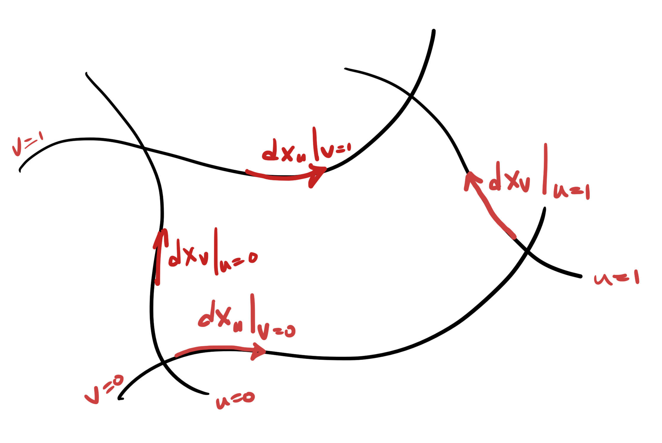
fig. 1. Two parameter manifold.

Our curvilinear coordinates \( \Bx_u, \Bx_v, \Bx_w \) are dual to the reciprocal basis \( \Bx^u, \Bx^v, \Bx^w \), but we won’t actually have to calculate that reciprocal basis. Instead we need only know that it can be calculated and is defined by the relations \( \Bx_a \cdot \Bx^b = \delta_a^b \). Knowing that we can reduce (say),

\begin{equation}\label{eqn:stokesMaxwellSpaceTimeSplit:140}
\begin{aligned}
d^2 \Bx \cdot ( \spacegrad \wedge \BE )
&=
d^2 \Bx \cdot ( \Bx^a \partial_a \wedge \BE ) \\
&=
(\Bx_u \wedge \Bx_v) \cdot ( \Bx^a \wedge \partial_a \BE ) \,du dv \\
&=
(((\Bx_u \wedge \Bx_v) \cdot \Bx^a) \cdot \partial_a \BE \,du dv \\
&=
d\Bx_u \cdot \partial_v \BE \,dv
-d\Bx_v \cdot \partial_u \BE \,du,
\end{aligned}
\end{equation}

Because each of the differentials, for example \( d\Bx_u = (\PDi{u}{\Bx}) du \), is calculated with the other (i.e.\( v \)) held constant, this is directly integrable, leaving

\begin{equation}\label{eqn:stokesMaxwellSpaceTimeSplit:160}
\begin{aligned}
\int d^2 \Bx \cdot ( \spacegrad \wedge \BE )
&=
\int \evalrange{\lr{d\Bx_u \cdot \BE}}{v=0}{v=1}
-\int \evalrange{\lr{d\Bx_v \cdot \BE}}{u=0}{u=1} \\
&=
\oint d\Bx \cdot \BE.
\end{aligned}
\end{equation}

That direct integration of one of the parameters, while the others are held constant, is the basic idea behind Stokes theorem.

The pseudoscalar grade Maxwell’s equations from \ref{eqn:stokesMaxwellSpaceTimeSplit:80} require a three parameter volume element to apply Stokes theorem to. Again, allowing for curvilinear coordinates such a differential expands as

\begin{equation}\label{eqn:stokesMaxwellSpaceTimeSplit:180}
\begin{aligned}
d^3 \Bx \cdot (\spacegrad \wedge (I\BB))
&=
(( \Bx_u \wedge \Bx_v \wedge \Bx_w ) \cdot \Bx^a ) \cdot \partial_a (I\BB) \,du dv dw \\
&=
(d\Bx_u \wedge d\Bx_v) \cdot \partial_w (I\BB) dw
+(d\Bx_v \wedge d\Bx_w) \cdot \partial_u (I\BB) du
+(d\Bx_w \wedge d\Bx_u) \cdot \partial_v (I\BB) dv.
\end{aligned}
\end{equation}

Like the two parameter volume, this is directly integrable

\begin{equation}\label{eqn:stokesMaxwellSpaceTimeSplit:200}
\int
d^3 \Bx \cdot (\spacegrad \wedge (I\BB))
=
\int \evalbar{(d\Bx_u \wedge d\Bx_v) \cdot (I\BB) }{\Delta w}
+\int \evalbar{(d\Bx_v \wedge d\Bx_w) \cdot (I\BB)}{\Delta u}
+\int \evalbar{(d\Bx_w \wedge d\Bx_u) \cdot (I\BB)}{\Delta v}.
\end{equation}

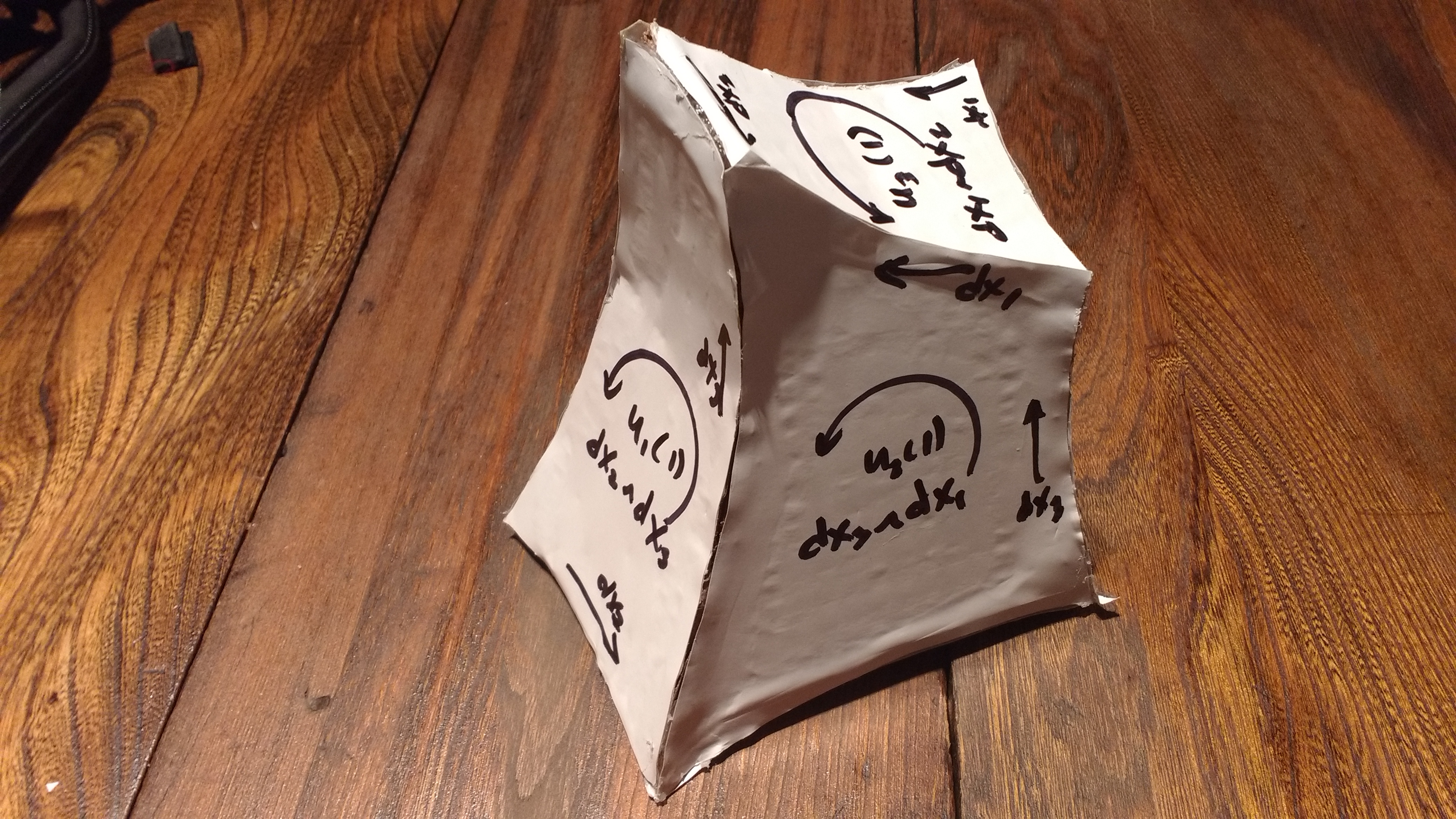
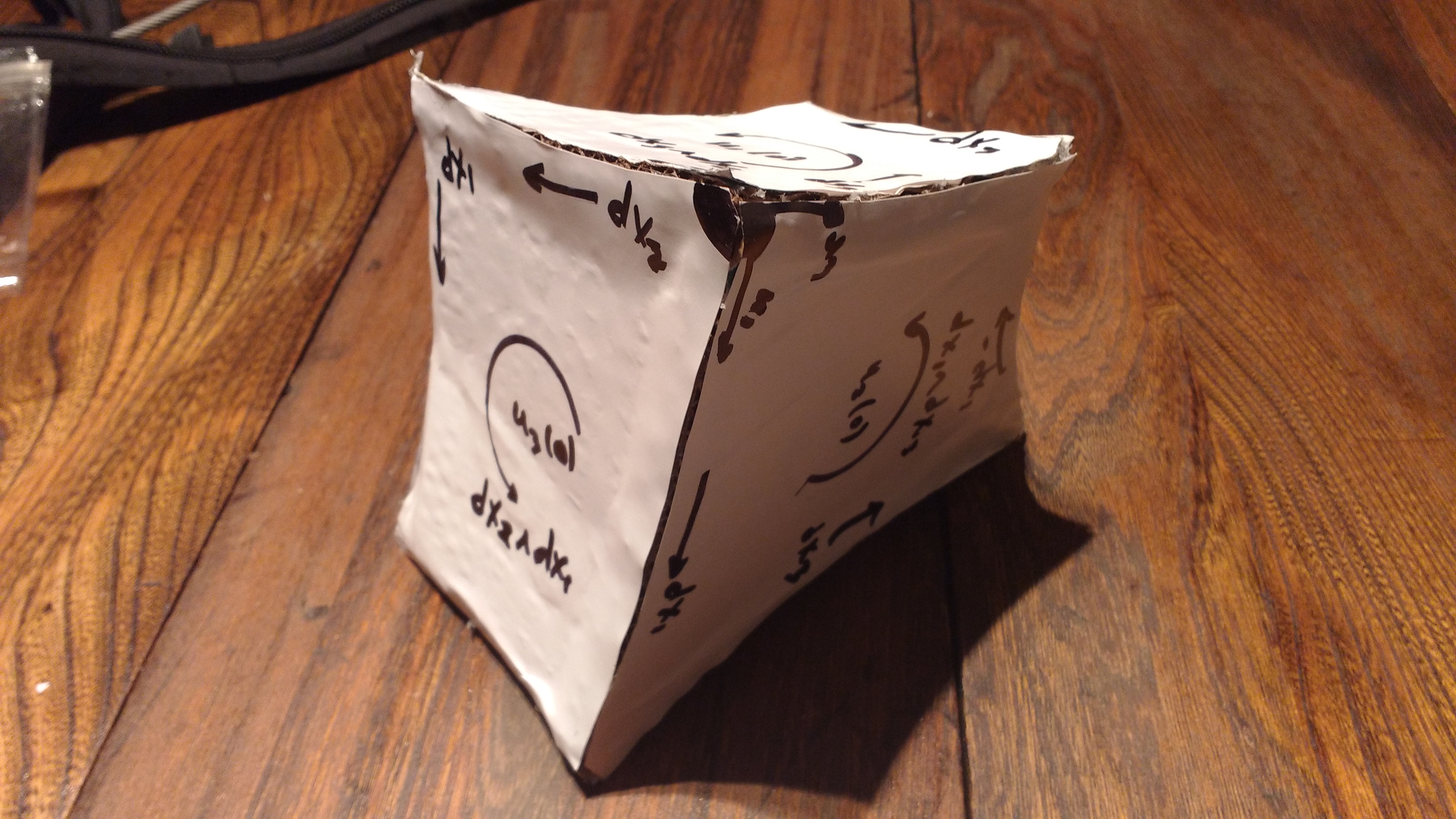
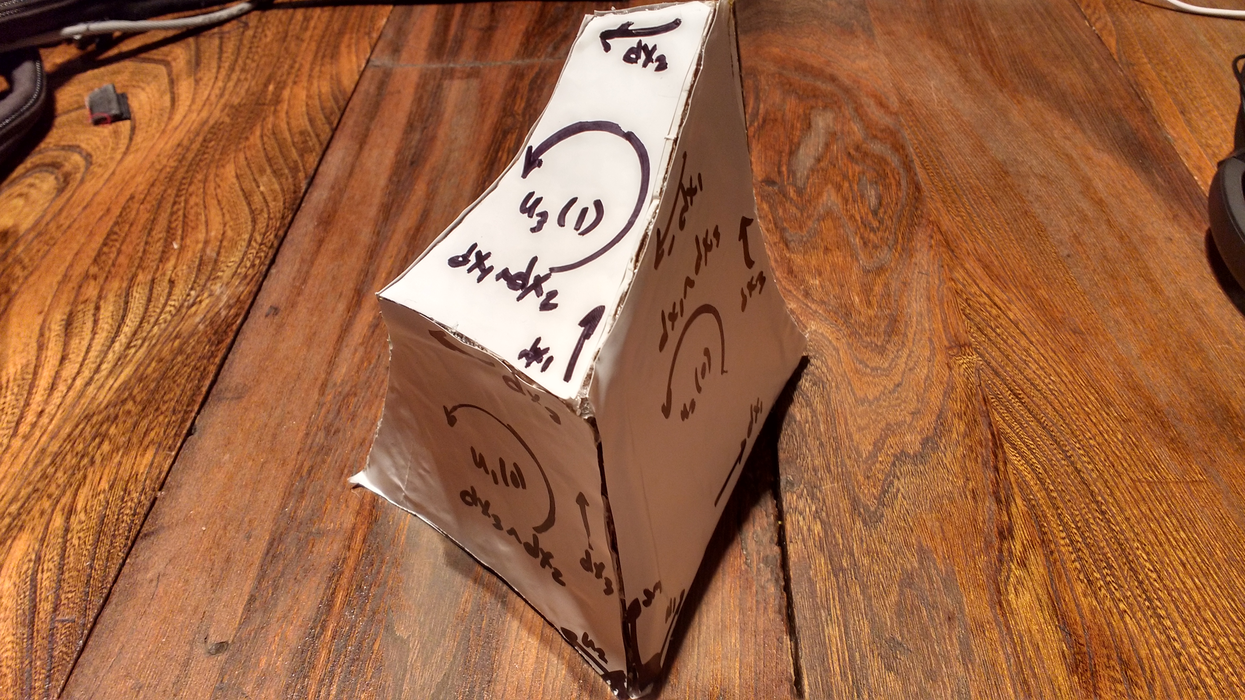
After some thought (or a craft project such as that of fig. 2) is can be observed that this is conceptually an oriented surface integral

threeParameterSurfaceFig2

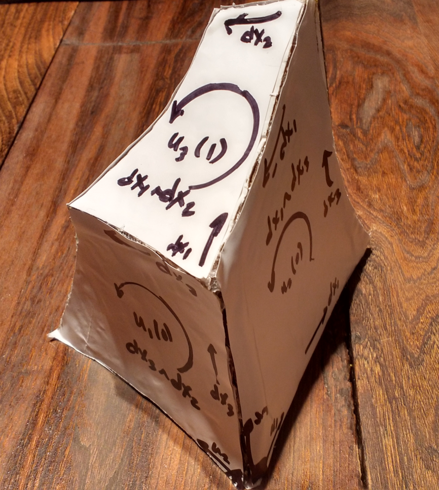
fig. 2. Oriented three parameter surface.

Noting that

\begin{equation}\label{eqn:stokesMaxwellSpaceTimeSplit:221}
\begin{aligned}
d^2 \Bx \cdot (I\Bf)
&= \gpgradezero{ d^2 \Bx I B } \\
&= I (d^2\Bx \wedge \Bf)
\end{aligned}
\end{equation}

we can now write down the results of application of Stokes theorem to each of Maxwell’s equations in their curl forms

\begin{equation}\label{eqn:stokesMaxwellSpaceTimeSplit:220}
\boxed{
\begin{aligned}
\oint d\Bx \cdot \BE &= -I \partial_t \int d^2 \Bx \wedge \BB \\
\inv{\mu_0} \oint d\Bx \cdot \BB &= \epsilon_0 I \partial_t \int d^2 \Bx \wedge \BE + I \int d^2 \Bx \wedge \BJ \\
\oint d^2 \Bx \wedge \BE &= \inv{\epsilon_0} \int (d^3 \Bx \cdot I) \rho \\
\oint d^2 \Bx \wedge \BB &= 0.
\end{aligned}
}
\end{equation}

In the three parameter surface integrals the specific meaning to apply to \( d^2 \Bx \wedge \Bf \) is
\begin{equation}\label{eqn:stokesMaxwellSpaceTimeSplit:240}
\oint d^2 \Bx \wedge \Bf
=
\int \evalbar{\lr{d\Bx_u \wedge d\Bx_v \wedge \Bf}}{\Delta w}
+\int \evalbar{\lr{d\Bx_v \wedge d\Bx_w \wedge \Bf}}{\Delta u}
+\int \evalbar{\lr{d\Bx_w \wedge d\Bx_u \wedge \Bf}}{\Delta v}.
\end{equation}

Note that in each case only the component of the vector \( \Bf \) that is projected onto the normal to the area element contributes.

Application of Stokes Theorem to the Maxwell equation

September 3, 2016 math and physics play , , , , , , , , , , , ,

[Click here for a PDF of this post with nicer formatting]

The relativistic form of Maxwell’s equation in Geometric Algebra is

\begin{equation}\label{eqn:maxwellStokes:20}
\grad F = \inv{c \epsilon_0} J,
\end{equation}

where \( \grad = \gamma^\mu \partial_\mu \) is the spacetime gradient, and \( J = (c\rho, \BJ) = J^\mu \gamma_\mu \) is the four (vector) current density. The pseudoscalar for the space is denoted \( I = \gamma_0 \gamma_1 \gamma_2 \gamma_3 \), where the basis elements satisfy \( \gamma_0^2 = 1 = -\gamma_k^2 \), and a dual basis satisfies \( \gamma_\mu \cdot \gamma^\nu = \delta_\mu^\nu \). The electromagnetic field \( F \) is a composite multivector \( F = \BE + I c \BB \). This is actually a bivector because spatial vectors have a bivector representation in the space time algebra of the form \( \BE = E^k \gamma_k \gamma_0 \).

A dual representation, with \( F = I G \) is also possible

\begin{equation}\label{eqn:maxwellStokes:60}
\grad G = \frac{I}{c \epsilon_0} J.
\end{equation}

Either form of Maxwell’s equation can be split into grade one and three components. The standard (non-dual) form is

\begin{equation}\label{eqn:maxwellStokes:40}
\begin{aligned}
\grad \cdot F &= \inv{c \epsilon_0} J \\
\grad \wedge F &= 0,
\end{aligned}
\end{equation}

and the dual form is

\begin{equation}\label{eqn:maxwellStokes:41}
\begin{aligned}
\grad \cdot G &= 0 \\
\grad \wedge G &= \frac{I}{c \epsilon_0} J.
\end{aligned}
\end{equation}

In both cases a potential representation \( F = \grad \wedge A \), where \( A \) is a four vector potential can be used to kill off the non-current equation. Such a potential representation reduces Maxwell’s equation to

\begin{equation}\label{eqn:maxwellStokes:80}
\grad \cdot F = \inv{c \epsilon_0} J,
\end{equation}

or
\begin{equation}\label{eqn:maxwellStokes:100}
\grad \wedge G = \frac{I}{c \epsilon_0} J.
\end{equation}

In both cases, these reduce to
\begin{equation}\label{eqn:maxwellStokes:120}
\grad^2 A – \grad \lr{ \grad \cdot A } = \inv{c \epsilon_0} J.
\end{equation}

This can clearly be further simplified by using the Lorentz gauge, where \( \grad \cdot A = 0 \). However, the aim for now is to try applying Stokes theorem to Maxwell’s equation. The dual form \ref{eqn:maxwellStokes:100} has the curl structure required for the application of Stokes. Suppose that we evaluate this curl over the three parameter volume element \( d^3 x = i\, dx^0 dx^1 dx^2 \), where \( i = \gamma_0 \gamma_1 \gamma_2 \) is the unit pseudoscalar for the spacetime volume element.

\begin{equation}\label{eqn:maxwellStokes:101}
\begin{aligned}
\int_V d^3 x \cdot \lr{ \grad \wedge G }
&=
\int_V d^3 x \cdot \lr{ \gamma^\mu \wedge \partial_\mu G } \\
&=
\int_V \lr{ d^3 x \cdot \gamma^\mu } \cdot \partial_\mu G \\
&=
\sum_{\mu \ne 3} \int_V \lr{ d^3 x \cdot \gamma^\mu } \cdot \partial_\mu G.
\end{aligned}
\end{equation}

This uses the distibution identity \( A_s \cdot (a \wedge A_r) = (A_s \cdot a) \cdot A_r \) which holds for blades \( A_s, A_r \) provided \( s > r > 0 \). Observe that only the component of the gradient that lies in the tangent space of the three volume manifold contributes to the integral, allowing the gradient to be used in the Stokes integral instead of the vector derivative (see: [1]).
Defining the the surface area element

\begin{equation}\label{eqn:maxwellStokes:140}
\begin{aligned}
d^2 x
&= \sum_{\mu \ne 3} i \cdot \gamma^\mu \inv{dx^\mu} d^3 x \\
&= \gamma_1 \gamma_2 dx dy
+ c \gamma_2 \gamma_0 dt dy
+ c \gamma_0 \gamma_1 dt dx,
\end{aligned}
\end{equation}

Stokes theorem for this volume element is now completely specified

\begin{equation}\label{eqn:maxwellStokes:200}
\int_V d^3 x \cdot \lr{ \grad \wedge G }
=
\int_{\partial V} d^2 \cdot G.
\end{equation}

Application to the dual Maxwell equation gives

\begin{equation}\label{eqn:maxwellStokes:160}
\int_{\partial V} d^2 x \cdot G
= \inv{c \epsilon_0} \int_V d^3 x \cdot (I J).
\end{equation}

After some manipulation, this can be restated in the non-dual form

\begin{equation}\label{eqn:maxwellStokes:180}
\boxed{
\int_{\partial V} \inv{I} d^2 x \wedge F
= \frac{1}{c \epsilon_0 I} \int_V d^3 x \wedge J.
}
\end{equation}

It can be demonstrated that using this with each of the standard basis spacetime 3-volume elements recovers Gauss’s law and the Ampere-Maxwell equation. So, what happened to Faraday’s law and Gauss’s law for magnetism? With application of Stokes to the curl equation from \ref{eqn:maxwellStokes:40}, those equations take the form

\begin{equation}\label{eqn:maxwellStokes:240}
\boxed{
\int_{\partial V} d^2 x \cdot F = 0.
}
\end{equation}

Problem 1:

Demonstrate that the Ampere-Maxwell equation and Gauss’s law can be recovered from the trivector (curl) equation \ref{eqn:maxwellStokes:100}.

Answer

The curl equation is a trivector on each side, so dotting it with each of the four possible trivectors \( \gamma_0 \gamma_1 \gamma_2, \gamma_0 \gamma_2 \gamma_3, \gamma_0 \gamma_1 \gamma_3, \gamma_1 \gamma_2 \gamma_3 \) will give four different scalar equations. For example, dotting with \( \gamma_0 \gamma_1 \gamma_2 \), we have for the curl side

\begin{equation}\label{eqn:maxwellStokes:460}
\begin{aligned}
\lr{ \gamma_0 \gamma_1 \gamma_2 } \cdot \lr{ \gamma^\mu \wedge \partial_\mu G }
&=
\lr{ \lr{ \gamma_0 \gamma_1 \gamma_2 } \cdot \gamma^\mu } \cdot \partial_\mu G \\
&=
(\gamma_0 \gamma_1) \cdot \partial_2 G
+(\gamma_2 \gamma_0) \cdot \partial_1 G
+(\gamma_1 \gamma_2) \cdot \partial_0 G,
\end{aligned}
\end{equation}

and for the current side, we have

\begin{equation}\label{eqn:maxwellStokes:480}
\begin{aligned}
\inv{\epsilon_0 c} \lr{ \gamma_0 \gamma_1 \gamma_2 } \cdot \lr{ I J }
&=
\inv{\epsilon_0 c} \gpgradezero{ \gamma_0 \gamma_1 \gamma_2 (\gamma_0 \gamma_1 \gamma_2 \gamma_3) J } \\
&=
\inv{\epsilon_0 c} \gpgradezero{ -\gamma_3 J } \\
&=
\inv{\epsilon_0 c} \gamma^3 \cdot J \\
&=
\inv{\epsilon_0 c} J^3,
\end{aligned}
\end{equation}

so we have
\begin{equation}\label{eqn:maxwellStokes:500}
(\gamma_0 \gamma_1) \cdot \partial_2 G
+(\gamma_2 \gamma_0) \cdot \partial_1 G
+(\gamma_1 \gamma_2) \cdot \partial_0 G
=
\inv{\epsilon_0 c} J^3.
\end{equation}

Similarily, dotting with \( \gamma_{013}, \gamma_{023}, and \gamma_{123} \) respectively yields
\begin{equation}\label{eqn:maxwellStokes:620}
\begin{aligned}
\gamma_{01} \cdot \partial_3 G + \gamma_{30} \partial_1 G + \gamma_{13} \partial_0 G &= – \inv{\epsilon_0 c} J^2 \\
\gamma_{02} \cdot \partial_3 G + \gamma_{30} \partial_2 G + \gamma_{23} \partial_0 G &= \inv{\epsilon_0 c} J^1 \\
\gamma_{12} \cdot \partial_3 G + \gamma_{31} \partial_2 G + \gamma_{23} \partial_1 G &= -\inv{\epsilon_0} \rho.
\end{aligned}
\end{equation}

Expanding the dual electromagnetic field, first in terms of the spatial vectors, and then in the space time basis, we have
\begin{equation}\label{eqn:maxwellStokes:520}
\begin{aligned}
G
&= -I F \\
&= -I \lr{ \BE + I c \BB } \\
&= -I \BE + c \BB. \\
&= -I \BE + c B^k \gamma_k \gamma_0 \\
&= \inv{2} \epsilon^{r s t} \gamma_r \gamma_s E^t + c B^k \gamma_k \gamma_0.
\end{aligned}
\end{equation}

So, dotting with a spatial vector will pick up a component of \( \BB \), we have
\begin{equation}\label{eqn:maxwellStokes:540}
\begin{aligned}
\lr{ \gamma_m \wedge \gamma_0 } \cdot \partial_\mu G
&=
\lr{ \gamma_m \wedge \gamma_0 } \cdot \partial_\mu \lr{
\inv{2} \epsilon^{r s t} \gamma_r \gamma_s E^t + c B^k \gamma_k \gamma_0
} \\
&=
c \partial_\mu B^k
\gpgradezero{
\gamma_m \gamma_0 \gamma_k \gamma_0
} \\
&=
c \partial_\mu B^k
\gpgradezero{
\gamma_m \gamma_0 \gamma_0 \gamma^k
} \\
&=
c \partial_\mu B^k
\delta_m^k \\
&=
c \partial_\mu B^m.
\end{aligned}
\end{equation}

Written out explicitly the electric field contributions to \( G \) are

\begin{equation}\label{eqn:maxwellStokes:560}
\begin{aligned}
-I \BE
&=
-\gamma_{0123k0} E^k \\
&=
-\gamma_{123k} E^k \\
&=
\left\{
\begin{array}{l l}
\gamma_{12} E^3 & \quad \mbox{\( k = 3 \)} \\
\gamma_{31} E^2 & \quad \mbox{\( k = 2 \)} \\
\gamma_{23} E^1 & \quad \mbox{\( k = 1 \)} \\
\end{array}
\right.,
\end{aligned}
\end{equation}

so
\begin{equation}\label{eqn:maxwellStokes:580}
\begin{aligned}
\gamma_{23} \cdot G &= -E^1 \\
\gamma_{31} \cdot G &= -E^2 \\
\gamma_{12} \cdot G &= -E^3.
\end{aligned}
\end{equation}

We now have the pieces required to expand \ref{eqn:maxwellStokes:500} and \ref{eqn:maxwellStokes:620}, which are respectively

\begin{equation}\label{eqn:maxwellStokes:501}
\begin{aligned}
– c \partial_2 B^1 + c \partial_1 B^2 – \partial_0 E^3 &= \inv{\epsilon_0 c} J^3 \\
– c \partial_3 B^1 + c \partial_1 B^3 + \partial_0 E^2 &= -\inv{\epsilon_0 c} J^2 \\
– c \partial_3 B^2 + c \partial_2 B^3 – \partial_0 E^1 &= \inv{\epsilon_0 c} J^1 \\
– \partial_3 E^3 – \partial_2 E^2 – \partial_1 E^1 &= – \inv{\epsilon_0} \rho
\end{aligned}
\end{equation}

which are the components of the Ampere-Maxwell equation, and Gauss’s law

\begin{equation}\label{eqn:maxwellStokes:600}
\begin{aligned}
\inv{\mu_0} \spacegrad \cross \BB – \epsilon_0 \PD{t}{\BE} &= \BJ \\
\spacegrad \cdot \BE &= \frac{\rho}{\epsilon_0}.
\end{aligned}
\end{equation}

Problem 2:

Prove \ref{eqn:maxwellStokes:180}.

Answer

The proof just requires the expansion of the dot products using scalar selection

\begin{equation}\label{eqn:maxwellStokes:260}
\begin{aligned}
d^2 x \cdot G
&=
\gpgradezero{ d^2 x (-I) F } \\
&=
-\gpgradezero{ I d^2 x F } \\
&=
-I \lr{ d^2 x \wedge F },
\end{aligned}
\end{equation}

and
for the three volume dot product

\begin{equation}\label{eqn:maxwellStokes:280}
\begin{aligned}
d^3 x \cdot (I J)
&=
\gpgradezero{
d^3 x\, I J
} \\
&=
-\gpgradezero{
I d^3 x\, J
} \\
&=
-I \lr{ d^3 x \wedge J }.
\end{aligned}
\end{equation}

Problem 3:

Using each of the four possible spacetime volume elements, write out the components of the Stokes integral
\ref{eqn:maxwellStokes:180}.

Answer

The four possible volume and associated area elements are
\begin{equation}\label{eqn:maxwellStokes:220}
\begin{aligned}
d^3 x = c \gamma_0 \gamma_1 \gamma_2 dt dx dy & \qquad d^2 x = \gamma_1 \gamma_2 dx dy + c \gamma_2 \gamma_0 dy dt + c \gamma_0 \gamma_1 dt dx \\
d^3 x = c \gamma_0 \gamma_1 \gamma_3 dt dx dz & \qquad d^2 x = \gamma_1 \gamma_3 dx dz + c \gamma_3 \gamma_0 dz dt + c \gamma_0 \gamma_1 dt dx \\
d^3 x = c \gamma_0 \gamma_2 \gamma_3 dt dy dz & \qquad d^2 x = \gamma_2 \gamma_3 dy dz + c \gamma_3 \gamma_0 dz dt + c \gamma_0 \gamma_2 dt dy \\
d^3 x = \gamma_1 \gamma_2 \gamma_3 dx dy dz & \qquad d^2 x = \gamma_1 \gamma_2 dx dy + \gamma_2 \gamma_3 dy dz + c \gamma_3 \gamma_1 dz dx \\
\end{aligned}
\end{equation}

Wedging the area element with \( F \) will produce pseudoscalar multiples of the various \( \BE \) and \( \BB \) components, but a recipe for these components is required.

First note that for \( k \ne 0 \), the wedge \( \gamma_k \wedge \gamma_0 \wedge F \) will just select components of \( \BB \). This can be seen first by simplifying

\begin{equation}\label{eqn:maxwellStokes:300}
\begin{aligned}
I \BB
&=
\gamma_{0 1 2 3} B^m \gamma_{m 0} \\
&=
\left\{
\begin{array}{l l}
\gamma_{3 2} B^1 & \quad \mbox{\( m = 1 \)} \\
\gamma_{1 3} B^2 & \quad \mbox{\( m = 2 \)} \\
\gamma_{2 1} B^3 & \quad \mbox{\( m = 3 \)}
\end{array}
\right.,
\end{aligned}
\end{equation}

or

\begin{equation}\label{eqn:maxwellStokes:320}
I \BB = – \epsilon_{a b c} \gamma_{a b} B^c.
\end{equation}

From this it follows that

\begin{equation}\label{eqn:maxwellStokes:340}
\gamma_k \wedge \gamma_0 \wedge F = I c B^k.
\end{equation}

The electric field components are easier to pick out. Those are selected by

\begin{equation}\label{eqn:maxwellStokes:360}
\begin{aligned}
\gamma_m \wedge \gamma_n \wedge F
&= \gamma_m \wedge \gamma_n \wedge \gamma_k \wedge \gamma_0 E^k \\
&= -I E^k \epsilon_{m n k}.
\end{aligned}
\end{equation}

The respective volume element wedge products with \( J \) are

\begin{equation}\label{eqn:maxwellStokes:400}
\begin{aligned}
\inv{I} d^3 x \wedge J = \inv{c \epsilon_0} J^3
\inv{I} d^3 x \wedge J = \inv{c \epsilon_0} J^2
\inv{I} d^3 x \wedge J = \inv{c \epsilon_0} J^1,
\end{aligned}
\end{equation}

and the respective sum of surface area elements wedged with the electromagnetic field are

\begin{equation}\label{eqn:maxwellStokes:380}
\begin{aligned}
\inv{I} d^2 x \wedge F &= – \evalbar{E^3}{c \Delta t} dx dy + c \lr{ \evalbar{B^2}{\Delta x} dy – \evalbar{B^1}{\Delta y} dx } dt \\
\inv{I} d^2 x \wedge F &= \evalbar{E^2}{c \Delta t} dx dz + c \lr{ \evalbar{B^3}{\Delta x} dz – \evalbar{B^1}{\Delta z} dx } dt \\
\inv{I} d^2 x \wedge F &= – \evalbar{E^1}{c \Delta t} dy dz + c \lr{ \evalbar{B^3}{\Delta y} dz – \evalbar{B^2}{\Delta z} dy } dt \\
\inv{I} d^2 x \wedge F &= – \evalbar{E^3}{\Delta z} dy dx – \evalbar{E^2}{\Delta y} dx dz – \evalbar{E^1}{\Delta x} dz dy,
\end{aligned}
\end{equation}

so
\begin{equation}\label{eqn:maxwellStokes:381}
\begin{aligned}
\int_{\partial V} – \evalbar{E^3}{c \Delta t} dx dy + c \lr{ \evalbar{B^2}{\Delta x} dy – \evalbar{B^1}{\Delta y} dx } dt &=
c \int_V dx dy dt \inv{c \epsilon_0} J^3 \\
\int_{\partial V} \evalbar{E^2}{c \Delta t} dx dz + c \lr{ \evalbar{B^3}{\Delta x} dz – \evalbar{B^1}{\Delta z} dx } dt &=
-c \int_V dx dy dt \inv{c \epsilon_0} J^2 \\
\int_{\partial V} – \evalbar{E^1}{c \Delta t} dy dz + c \lr{ \evalbar{B^3}{\Delta y} dz – \evalbar{B^2}{\Delta z} dy } dt &=
c \int_V dx dy dt \inv{c \epsilon_0} J^1 \\
\int_{\partial V} – \evalbar{E^3}{\Delta z} dy dx – \evalbar{E^2}{\Delta y} dx dz – \evalbar{E^1}{\Delta x} dz dy &=
-\int_V dx dy dz \inv{\epsilon_0} \rho.
\end{aligned}
\end{equation}

Observe that if the volume elements are taken to their infinesimal limits, we recover the traditional differential forms of the Ampere-Maxwell and Gauss’s law equations.

References

[1] A. Macdonald. Vector and Geometric Calculus. CreateSpace Independent Publishing Platform, 2012.

Electric field due to spherical shell

August 24, 2016 math and physics play , ,

[Click here for a PDF of this post with nicer formatting]

Here’s a problem (2.7) from [1], to calculate the field due to a spherical shell. The field is

\begin{equation}\label{eqn:griffithsEM2_7:20}
\BE = \frac{\sigma}{4 \pi \epsilon_0} \int \frac{(\Br – \Br’)}{\Abs{\Br – \Br’}^3} da’,
\end{equation}

where \( \Br’ \) is the position to the area element on the shell. For the test position, let \( \Br = z \Be_3 \). We need to parameterize the area integral. A complex-number like geometric algebra representation works nicely.

\begin{equation}\label{eqn:griffithsEM2_7:40}
\begin{aligned}
\Br’
&= R \lr{ \sin\theta \cos\phi, \sin\theta \sin\phi, \cos\theta } \\
&= R \lr{ \Be_1 \sin\theta \lr{ \cos\phi + \Be_1 \Be_2 \sin\phi } + \Be_3 \cos\theta } \\
&= R \lr{ \Be_1 \sin\theta e^{i\phi} + \Be_3 \cos\theta }.
\end{aligned}
\end{equation}

Here \( i = \Be_1 \Be_2 \) has been used to represent to horizontal rotation plane.

The difference in position between the test vector and area-element is

\begin{equation}\label{eqn:griffithsEM2_7:60}
\Br – \Br’
= \Be_3 \lr{ z – R \cos\theta } – R \Be_1 \sin\theta e^{i \phi},
\end{equation}

with an absolute squared length of

\begin{equation}\label{eqn:griffithsEM2_7:80}
\begin{aligned}
\Abs{\Br – \Br’ }^2
&= \lr{ z – R \cos\theta }^2 + R^2 \sin^2\theta \\
&= z^2 + R^2 – 2 z R \cos\theta.
\end{aligned}
\end{equation}

As a side note, this is a kind of fun way to prove the old “cosine-law” identity. With that done, the field integral can now be expressed explicitly

\begin{equation}\label{eqn:griffithsEM2_7:100}
\begin{aligned}
\BE
&= \frac{\sigma}{4 \pi \epsilon_0} \int_{\phi = 0}^{2\pi} \int_{\theta = 0}^\pi R^2 \sin\theta d\theta d\phi
\frac{\Be_3 \lr{ z – R \cos\theta } – R \Be_1 \sin\theta e^{i \phi}}
{
\lr{z^2 + R^2 – 2 z R \cos\theta}^{3/2}
} \\
&= \frac{2 \pi R^2 \sigma \Be_3}{4 \pi \epsilon_0} \int_{\theta = 0}^\pi \sin\theta d\theta
\frac{z – R \cos\theta}
{
\lr{z^2 + R^2 – 2 z R \cos\theta}^{3/2}
} \\
&= \frac{2 \pi R^2 \sigma \Be_3}{4 \pi \epsilon_0} \int_{\theta = 0}^\pi \sin\theta d\theta
\frac{ R( z/R – \cos\theta) }
{
(R^2)^{3/2} \lr{ (z/R)^2 + 1 – 2 (z/R) \cos\theta}^{3/2}
} \\
&= \frac{\sigma \Be_3}{2 \epsilon_0} \int_{u = -1}^{1} du
\frac{ z/R – u}
{
\lr{1 + (z/R)^2 – 2 (z/R) u}^{3/2}
}.
\end{aligned}
\end{equation}

Observe that all the azimuthal contributions get killed. We expect that due to the symmetry of the problem. We are left with an integral that submits to Mathematica, but doesn’t look fun to attempt manually. Specifically

\begin{equation}\label{eqn:griffithsEM2_7:120}
\int_{-1}^1 \frac{a-u}{\lr{1 + a^2 – 2 a u}^{3/2}} du
=
\left\{
\begin{array}{l l}
\frac{2}{a^2} & \quad \mbox{if \( a > 1 \) } \\
0 & \quad \mbox{if \( a < 1 \) } \end{array} \right., \end{equation} so \begin{equation}\label{eqn:griffithsEM2_7:140} \boxed{ \BE = \left\{ \begin{array}{l l} \frac{\sigma (R/z)^2 \Be_3}{\epsilon_0} & \quad \mbox{if \( z > R \) } \\
0 & \quad \mbox{if \( z < R \) } \end{array} \right. } \end{equation} In the problem, it is pointed out to be careful of the sign when evaluating \( \sqrt{ R^2 + z^2 - 2 R z } \), however, I don't see where that is even useful?

References

[1] David Jeffrey Griffiths and Reed College. Introduction to electrodynamics. Prentice hall Upper Saddle River, NJ, 3rd edition, 1999.

Geeking out: Oriented surface of volume element

August 20, 2016 math and physics play

Reading the intro chapters to my Griffiths electrodynamics, I ended up re-deriving the 1,2 and 3 parameter variations of Stokes Theorem (a quick derivation as previously done using Geometric Algebra [PDF], but without looking at my notes).  To understand how to map from the algebraic representation to a geometric one for the 3 parameter volume element, I built the following nice little model:IMG_20160820_231303757 IMG_20160820_231333998 IMG_20160820_231316618_HDR

This is like Fig 1.10 from the pdf notes linked above, but was a lot more fun to construct than the drawing.

Variational principle with two by two symmetric matrix

March 12, 2016 math and physics play , ,

[Click here for a PDF of this post with nicer formatting]

I pulled [1], one of too many lonely Dover books, off my shelf and started reading the review chapter. It posed the following question, which I thought had an interesting subquestion.

Variational principle with two by two matrix.

Consider a \( 2 \times 2 \) real symmetric matrix operator \(\BO \), with an arbitrary normalized trial vector

\begin{equation}\label{eqn:variationalMatrix:20}
\Bc =
\begin{bmatrix}
\cos\theta \\
\sin\theta
\end{bmatrix}.
\end{equation}

The variational principle requires that minimum value of \( \omega(\theta) = \Bc^\dagger \BO \Bc \) is greater than or equal to the lowest eigenvalue. If that minimum value occurs at \( \omega(\theta_0) \), show that this is exactly equal to the lowest eigenvalue and explain why this is expected.

Why this is expected is the part of the question that I thought was interesting.

Finding the minimum.

If the operator representation is

\begin{equation}\label{eqn:variationalMatrix:40}
\BO =
\begin{bmatrix}
a & b \\
b & d
\end{bmatrix},
\end{equation}

then the variational product is

\begin{equation}\label{eqn:variationalMatrix:80}
\begin{aligned}
\omega(\theta)
&=
\begin{bmatrix}
\cos\theta & \sin\theta
\end{bmatrix}
\begin{bmatrix}
a & b \\
b & d
\end{bmatrix}
\begin{bmatrix}
\cos\theta \\
\sin\theta
\end{bmatrix} \\
&=
\begin{bmatrix}
\cos\theta & \sin\theta
\end{bmatrix}
\begin{bmatrix}
a \cos\theta + b \sin\theta \\
b \cos\theta + d \sin\theta
\end{bmatrix} \\
&=
a \cos^2\theta + 2 b \sin\theta \cos\theta
+ d \sin^2\theta \\
&=
a \cos^2\theta + b \sin( 2 \theta )
+ d \sin^2\theta.
\end{aligned}
\end{equation}

The minimum is given by

\begin{equation}\label{eqn:variationalMatrix:60}
\begin{aligned}
0
&=
\frac{d\omega}{d\theta} \\
&=
-2 a \sin\theta \cos\theta + 2 b \cos( 2 \theta )
+ 2 d \sin\theta \cos\theta \\
&=
2 b \cos( 2 \theta )
+ (d -a)\sin( 2 \theta )
\end{aligned}
,
\end{equation}

so the extreme values will be found at

\begin{equation}\label{eqn:variationalMatrix:100}
\tan(2\theta_0) = \frac{2 b}{a – d}.
\end{equation}

Solving for \( \cos(2\theta_0) \), with \( \alpha = 2b/(a-d) \), we have

\begin{equation}\label{eqn:variationalMatrix:120}
1 – \cos^2(2\theta) = \alpha^2 \cos^2(2 \theta),
\end{equation}

or

\begin{equation}\label{eqn:variationalMatrix:140}
\begin{aligned}
\cos^2(2\theta_0)
&= \frac{1}{1 + \alpha^2} \\
&= \frac{1}{1 + 4 b^2/(a-d)^2 } \\
&= \frac{(a-d)^2}{(a-d)^2 + 4 b^2 }.
\end{aligned}
\end{equation}

So,

\begin{equation}\label{eqn:variationalMatrix:200}
\begin{aligned}
\cos(2 \theta_0) &= \frac{ \pm (a-d) }{\sqrt{ (a-d)^2 + 4 b^2 }} \\
\sin(2 \theta_0) &= \frac{ \pm 2 b }{\sqrt{ (a-d)^2 + 4 b^2 }},
\end{aligned}
\end{equation}

Substituting this back into \( \omega(\theta_0) \) is a bit tedious.
I did it once on paper, then confirmed with Mathematica (quantumchemistry/twoByTwoSymmetricVariation.nb). The end result is

\begin{equation}\label{eqn:variationalMatrix:160}
\omega(\theta_0)
=
\inv{2} \lr{ a + d \pm \sqrt{ (a-d)^2 + 4 b^2 } }.
\end{equation}

The eigenvalues of the operator are given by

\begin{equation}\label{eqn:variationalMatrix:220}
\begin{aligned}
0
&= (a-\lambda)(d-\lambda) – b^2 \\
&= \lambda^2 – (a+d) \lambda + a d – b^2 \\
&= \lr{\lambda – \frac{a+d}{2}}^2 -\lr{ \frac{a+d}{2}}^2 + a d – b^2 \\
&= \lr{\lambda – \frac{a+d}{2}}^2 – \inv{4} \lr{ (a-d)^2 + 4 b^2 },
\end{aligned}
\end{equation}

so the eigenvalues are exactly the values \ref{eqn:variationalMatrix:160} as stated by the problem statement.

Why should this have been anticipated?

If the eigenvectors are \( \Be_1, \Be_2 \), the operator can be diagonalized as

\begin{equation}\label{eqn:variationalMatrix:240}
\BO = U D U^\T,
\end{equation}

where \( U = \begin{bmatrix} \Be_1 & \Be_2 \end{bmatrix} \), and \( D \) has the eigenvalues along the diagonal. The energy function \( \omega \) can now be written

\begin{equation}\label{eqn:variationalMatrix:260}
\begin{aligned}
\omega
&= \Bc^\T U D U^\T \Bc \\
&= (U^\T \Bc)^\T D U^\T \Bc.
\end{aligned}
\end{equation}

We can show that the transformed vector \( U^\T \Bc \) is still a unit vector

\begin{equation}\label{eqn:variationalMatrix:280}
\begin{aligned}
U^\T \Bc
&=
\begin{bmatrix}
\Be_1^\T \\
\Be_2^\T \\
\end{bmatrix}
\Bc \\
&=
\begin{bmatrix}
\Be_1^\T \Bc \\
\Be_2^\T \Bc \\
\end{bmatrix},
\end{aligned}
\end{equation}

so
\begin{equation}\label{eqn:variationalMatrix:300}
\begin{aligned}
\Abs{
U^\T \Bc
}^2
&=
\Bc^\T \Be_1
\Be_1^\T \Bc
+
\Bc^\T \Be_2
\Be_2^\T \Bc \\
&=
\Bc^\T \lr{ \Be_1 \Be_1^\T
+
\Be_2
\Be_2^\T } \Bc \\
&=
\Bc^\T \Bc \\
&= 1,
\end{aligned}
\end{equation}

so the transformed vector can be written as

\begin{equation}\label{eqn:variationalMatrix:320}
U^\T \Bc =
\begin{bmatrix}
\cos\phi \\
\sin\phi
\end{bmatrix},
\end{equation}

for some \( \phi \). With such a representation we have
\begin{equation}\label{eqn:variationalMatrix:340}
\begin{aligned}
\omega
&=
\begin{bmatrix}
\cos\phi & \sin\phi
\end{bmatrix}
\begin{bmatrix}
\lambda_1 & 0 \\
0 & \lambda_2
\end{bmatrix}
\begin{bmatrix}
\cos\phi \\
\sin\phi
\end{bmatrix} \\
&=
\begin{bmatrix}
\cos\phi & \sin\phi
\end{bmatrix}
\begin{bmatrix}
\lambda_1 \cos\phi \\
\lambda_2 \sin\phi
\end{bmatrix} \\
&=
\lambda_1 \cos^2\phi + \lambda_2 \sin^2\phi.
\end{aligned}
\end{equation}

This has it’s minimums where \( 0 = \sin(2 \phi)( \lambda_2 – \lambda_1 ) \). For the non-degenerate case, two zeros at \( \phi = n \pi/2 \) for integral \( n \). For \( \phi = 0, \pi/2 \), we have

\begin{equation}\label{eqn:variationalMatrix:360}
\Bc =
\begin{bmatrix}
1 \\
0
\end{bmatrix},
\begin{bmatrix}
0 \\
1
\end{bmatrix}.
\end{equation}

We see that the extreme values of \( \omega \) occur when the trial vectors \( \Bc \) are eigenvectors of the operator.

References

[1] Attila Szabo and Neil S Ostlund. Modern quantum chemistry: introduction to advanced electronic structure theory. Dover publications, 1989.