Singular Value Decomposition

October 2, 2014 ece1254 , , , ,

[Click here for a PDF of this post with nicer formatting]

We’ve been presented with the definition of the singular value decomposition or SVD, but not how to compute it.

Recall that the definition was

Singular value decomposition (SVD)

Given \( M \in \text{R}^{m \times n} \), we can find a representation of \( M \)

\begin{equation}\label{eqn:svdNotes:81}
M = U \Sigma V^\T,
\end{equation}

where \( U \) and \( V\) are orthogonal matrices such that \( U^\T U = 1 \), and \( V^\T V = 1 \), and

\begin{equation}\label{eqn:svdNotes:101}
\Sigma =
\begin{bmatrix}
\sigma_1 & & & & & &\\
& \sigma_2 & & & & &\\
& & \ddots & & & &\\
& & & \sigma_r & & &\\
& & & & 0 & & \\
& & & & & \ddots & \\
& & & & & & 0 \\
\end{bmatrix}
\end{equation}

The values \( \sigma_i, i \le \min(n,m) \) are called the singular values of \( M \). The singular values are subject to the ordering

\begin{equation}\label{eqn:svdNotes:261}
\sigma_{1} \ge \sigma_{2} \ge \cdots \ge 0
\end{equation}

If \(r\) is the rank of \( M \), then the \( \sigma_r \) above is the minimum non-zero singular value (but the zeros are also called singular values).

Here I’ll review some of the key ideas from the MIT OCW SVD lecture by Prof. Gilbert Strang. This is largely to avoid having to rewatch this again in a few years as I just did.

The idea behind the SVD is to find an orthogonal basis that relates the image space of the transformation, as well as the basis for the vectors that the transformation applies to. That is a relation of the form

\begin{equation}\label{eqn:svdNotes:281}
\Bu_i = M \Bv_j
\end{equation}

Where \( \Bv_j \) are orthonormal basis vectors, and \( \Bu_i \) are orthonormal basis vectors for the image space. %Strang’s lectures call these the row and column spaces (or reverse?)

Let’s suppose that such a set of vectors can be computed and that \( M \) has a representation of the desired form

\begin{equation}\label{eqn:svdNotes:301}
M = U \Sigma V^\conj
\end{equation}

where
\begin{equation}\label{eqn:svdNotes:321}
U =
\begin{bmatrix}
\Bu_1 & \Bu_2 & \cdots & \Bu_m
\end{bmatrix},
\end{equation}

and

\begin{equation}\label{eqn:svdNotes:341}
V =
\begin{bmatrix}
\Bv_1 & \Bv_2 & \cdots & \Bv_n
\end{bmatrix}.
\end{equation}

By left or right multiplication of \( M \) with its (conjugate) transpose, we will see that the decomposed form of these products have a very simple form

\begin{equation}\label{eqn:svdNotes:361}
M^\conj M
=
V \Sigma^\conj U^\conj U \Sigma V^\conj
=
V \Sigma^\conj \Sigma V^\conj,
\end{equation}
\begin{equation}\label{eqn:svdNotes:381}
M M^\conj
=
U \Sigma V^\conj V \Sigma^\conj U^\conj
=
U \Sigma \Sigma^\conj U^\conj.
\end{equation}

Because \( \Sigma \) is diagonal, the products \( \Sigma^\conj \Sigma \) and \( \Sigma \Sigma^\conj \) are also both diagonal, and populated with the absolute squares of the singular values that we have presumed to exist. Because \( \Sigma \Sigma^\conj \) is an \( m \times m \) matrix, whereas \( \Sigma^\conj \Sigma \) is an \( n \times n \) matrix, so the numbers of zeros in each of these will differ, but each will have the structure

\begin{equation}\label{eqn:svdNotes:401}
\Sigma^\conj \Sigma \sim \Sigma \Sigma^\conj \sim
\begin{bmatrix}
\Abs{\sigma_1}^2 & & & & & &\\
& \Abs{ \sigma_2 }^2 & & & & &\\
& & \ddots & & & &\\
& & & \Abs{ \sigma_r }^2 & & &\\
& & & & 0 & & \\
& & & & & \ddots & \\
& & & & & & 0 \\
\end{bmatrix}
\end{equation}

This shows us one method of computing the singular value decomposition (for full rank systems), because we need only solve for the eigensystem of either \( M M^\conj \) or \( M^\conj M \) to find the singular values, and one of \( U \) or \( V \). To form \( U \) we will be able to find \( r \) orthonormal eigenvectors of \( M M^\conj \) and then supplement that with a mutually orthonormal set of vectors from the Null space of \( M \). We can form \( \Sigma \) by taking the square roots of the eigenvalues of \( M M^\conj \). With both \( \Sigma \) and \( U \) computed, we can then compute \( V \) by inversion. We could similarly solve for \( \Sigma \) and \( V \) by computing the eigensystem of \( M^\conj M \) and similarly supplementing those eigenvectors with vectors from the null space, and then compute \( U \) by inversion.

Let’s work the examples from the lecture to see how this works.

Example: Full rank 2×2 matrix

In the lecture the SVD decomposition is computed for

\begin{equation}\label{eqn:svdNotes:421}
M =
\begin{bmatrix}
4 & 4 \\
3 & -3
\end{bmatrix}
\end{equation}

For this we have

\begin{equation}\label{eqn:svdNotes:441}
M M^\conj
=
\begin{bmatrix}
32 & 0 \\
0 & 18
\end{bmatrix}
\end{equation}
\begin{equation}\label{eqn:svdNotes:461}
M^\conj M
=
\begin{bmatrix}
25 & 7 \\
7 & 25
\end{bmatrix}
\end{equation}

The first is already diagonalized so \( U = I \), and the singular values are found by inspection \( \{ \sqrt{32}, \sqrt{18} \} \), or

\begin{equation}\label{eqn:svdNotes:541}
\Sigma =
\begin{bmatrix}
\sqrt{32} & 0 \\
0 & \sqrt{18}
\end{bmatrix}
\end{equation}

Because the system is full rank we can solve for \( V \) by inversion

\begin{equation}\label{eqn:svdNotes:481}
\Sigma^{-1} U^\conj M = V^\conj,
\end{equation}

or
\begin{equation}\label{eqn:svdNotes:501}
V = M^\conj U \lr{ \Sigma^{-1} }^\conj.
\end{equation}

In this case that is

\begin{equation}\label{eqn:svdNotes:521}
V = \inv{\sqrt{2}}
\begin{bmatrix}
1 & 1 \\
1 & -1
\end{bmatrix}
\end{equation}

We could alternately compute \( V \) directly by diagonalizing \( M^\conj M \). We see that the eigenvectors are \( \lr{ 1, \pm 1 }/\sqrt{2} \), with respective eigenvalues \( \{ 32, 18 \} \).

This gives us \ref{eqn:svdNotes:541} and \ref{eqn:svdNotes:521}. Again, because the system is full rank, we can compute \( U \) by inversion. That is

\begin{equation}\label{eqn:svdNotes:561}
U = M V \Sigma^{-1}.
\end{equation}

Carrying out this calculation recovers \( U = I \) as expected. Looks like I used a different matrix than Prof. Strang used in his lecture (alternate signs on the 3’s). He had some trouble that arrived from independent calculation of the respective eigenspaces. Calculating one from the other avoids that trouble since there are different signed eigenvalues that can be chosen, and we are looking for specific mappings between the eigenspaces that satisfy the \( \Bu_i = M \Bv_j \) constraints encoded by the relationship \( M = U \Sigma V^\conj \).

Let’s work a non-full rank example, as in the lecture.

Example: 2×2 matrix without full rank

How about

\begin{equation}\label{eqn:svdNotes:581}
M =
\begin{bmatrix}
1 & 1 \\
2 & 2
\end{bmatrix}.
\end{equation}

For this we have

\begin{equation}\label{eqn:svdNotes:601}
M^\conj M =
\begin{bmatrix}
5 & 5 \\
5 & 5
\end{bmatrix}
\end{equation}
\begin{equation}\label{eqn:svdNotes:621}
M M^\conj =
\begin{bmatrix}
2 & 4 \\
4 & 8
\end{bmatrix}
\end{equation}

For which the non-zero eigenvalue is \( 10 \) and the corresponding eigenvalue is
\begin{equation}\label{eqn:svdNotes:641}
\Bv =
\inv{\sqrt{2}}
\begin{bmatrix}
1 \\
1
\end{bmatrix}.
\end{equation}

This gives us

\begin{equation}\label{eqn:svdNotes:661}
\Sigma =
\begin{bmatrix}
\sqrt{10} & 0 \\
0 & 0
\end{bmatrix}
\end{equation}

Since we require \( V \) to be orthonormal, there is only one choice (up to a sign) for the vector from the null space.

Let’s try

\begin{equation}\label{eqn:svdNotes:681}
V =
\inv{\sqrt{2}}
\begin{bmatrix}
1 & 1 \\
1 & -1
\end{bmatrix}
\end{equation}

We find that \( M M^\conj \) has eigenvalues \( \{ 10, 0 \} \) as expected. The eigenvector for the non-zero eigenvalue is found to be

\begin{equation}\label{eqn:svdNotes:701}
\Bu = \inv{\sqrt{5}}
\begin{bmatrix}
1 \\
2
\end{bmatrix}.
\end{equation}

It’s easy to expand this to an orthonormal basis, but do we have to pick a specific sign relative to the choice that we’ve made for \( V \)?

Let’s try

\begin{equation}\label{eqn:svdNotes:721}
U = \inv{\sqrt{5}}
\begin{bmatrix}
1 & 2 \\
2 & -1
\end{bmatrix}.
\end{equation}

Multiplying out \( U \Sigma V^\conj \) we have

\begin{equation}\label{eqn:svdNotes:741}
\begin{aligned}
\inv{\sqrt{5}}
\begin{bmatrix}
1 & 2 \\
2 & -1
\end{bmatrix}
\begin{bmatrix}
\sqrt{10} & 0 \\
0 & 0
\end{bmatrix}
\inv{\sqrt{2}}
\begin{bmatrix}
1 & 1 \\
1 & -1
\end{bmatrix}
&=
\begin{bmatrix}
1 & 2 \\
2 & -1
\end{bmatrix}
\begin{bmatrix}
1 & 0 \\
0 & 0
\end{bmatrix}
\begin{bmatrix}
1 & 1 \\
1 & -1
\end{bmatrix} \\
&=
\begin{bmatrix}
1 & 0 \\
2 & 0
\end{bmatrix}
\begin{bmatrix}
1 & 1 \\
1 & -1
\end{bmatrix} \\
&=
\begin{bmatrix}
1 & 1 \\
2 & 2
\end{bmatrix}.
\end{aligned}
\end{equation}

It appears that this works, although we haven’t demonstrated why that should be, and we could have gotten lucky with signs. There’s some theoretical work to do here, but let’s leave that for another day (or rely on software to do this computational task).

ECE1254H Modeling of Multiphysics Systems. Lecture 6: Singular value decomposition, and conditioning number. Taught by Prof. Piero Triverio

October 1, 2014 ece1254 , , , , ,

[Click here for a PDF of this post with nicer formatting]

Disclaimer

Peeter’s lecture notes from class. These may be incoherent and rough.

Matrix norm

We’ve defined the matrix norm of \( M \), for the system \( \overline{{y}} = M \overline{{x}} \) as

\begin{equation}\label{eqn:multiphysicsL6:21}
\Norm{M} = \max_{\Norm{\overline{{x}}} = 1} \Norm{ M \overline{{x}} }.
\end{equation}

We will typically use the \( L_2 \) norm, so that the matrix norm is
\begin{equation}\label{eqn:multiphysicsL6:41}
\Norm{M}_2 = \max_{\Norm{\overline{{x}}}_2 = 1} \Norm{ M \overline{{x}} }_2.
\end{equation}

It can be shown that

\begin{equation}\label{eqn:multiphysicsL6:61}
\Norm{M}_2 = \max_i \sigma_i(M),
\end{equation}

where \( \sigma_i(M) \) are the (SVD) singular values.

Singular value decomposition (SVD)

Given \( M \in R^{m \times n} \), we can find a representation of \( M \)

\begin{equation}\label{eqn:multiphysicsL6:81}
M = U \Sigma V^\T,
\end{equation}

where \( U \) and \( V\) are orthogonal matrices such that \( U^\T U = 1 \), and \( V^\T V = 1 \), and

\begin{equation}\label{eqn:multiphysicsL6:101}
\Sigma =
\begin{bmatrix}
\sigma_1 & & & & & &\\
& \sigma_2 & & & & &\\
& & \ddots & & & &\\
& & & \sigma_r & & &\\
& & & & 0 & & \\
& & & & & \ddots & \\
& & & & & & 0 \\
\end{bmatrix}
\end{equation}

The values \( \sigma_i, i \le \min(n,m) \) are called the singular values of \( M \). The singular values are subject to the ordering

\begin{equation}\label{eqn:multiphysicsL6:261}
\sigma_{1} \ge \sigma_{2} \ge \cdots \ge 0
\end{equation}

If \(r\) is the rank of \( M \), then the \( \sigma_r \) above is the minimum non-zero singular value (but the zeros are also called singular values).

Observe that the condition \( U^\T U = 1 \) is a statement of orthonormality. In terms of column vectors \( \overline{{u}}_i \), such a product written out explicitly is

\begin{equation}\label{eqn:multiphysicsL6:301}
\begin{bmatrix}
\overline{{u}}_1^\T \\ \overline{{u}}_2^\T \\ \vdots \\ \overline{{u}}_m^\T
\end{bmatrix}
\begin{bmatrix}
\overline{{u}}_1 & \overline{{u}}_2 & \cdots & \overline{{u}}_m
\end{bmatrix}
=
\begin{bmatrix}
1 & & & \\
& 1 & & \\
& & \ddots & \\
& & & 1
\end{bmatrix}.
\end{equation}

This is both normality \( \overline{{u}}_i^\T \overline{{u}}_i = 1 \), and orthonormality \( \overline{{u}}_i^\T \overline{{u}}_j = 1, i \ne j \).

Example: 2 x 2 case

(for column vectors \( \overline{{u}}_i, \overline{{v}}_j \)).

\begin{equation}\label{eqn:multiphysicsL6:281}
M =
\begin{bmatrix}
\overline{{u}}_1 & \overline{{u}}_2
\end{bmatrix}
\begin{bmatrix}
\sigma_1 & \\
& \sigma_2
\end{bmatrix}
\begin{bmatrix}
\overline{{v}}_1^\T \\
\overline{{v}}_2^\T
\end{bmatrix}
\end{equation}

Consider \( \overline{{y}} = M \overline{{x}} \), and take an \( \overline{{x}} \) with \( \Norm{\overline{{x}}}_2 = 1 \)

Note: I’ve chosen not to sketch what was drawn on the board. See instead the animated gif of the same in \citep{wiki:svd}.

A very nice video treatment of SVD by Prof Gilbert Strang can be found in \citep{ocw:svd}.

Conditioning number

Given a perturbation of \( M \overline{{x}} = \overline{{b}} \) to

\begin{equation}\label{eqn:multiphysicsL6:121}
\lr{ M + \delta M }
\lr{ \overline{{x}} + \delta \overline{{x}} } = \overline{{b}},
\end{equation}

or
\begin{equation}\label{eqn:multiphysicsL6:141}
\underbrace{ M \overline{{x}} – \overline{{b}} }_{=0} + \delta M \overline{{x}} + M \delta \overline{{x}} + \delta M \delta \overline{{x}} = 0.
\end{equation}

This gives

\begin{equation}\label{eqn:multiphysicsL6:161}
M \delta \overline{{x}} = – \delta M \overline{{x}} – \delta M \delta \overline{{x}},
\end{equation}

or
\begin{equation}\label{eqn:multiphysicsL6:181}
\delta \overline{{x}} = – M^{-1} \delta M \lr{ \overline{{x}} + \delta \overline{{x}} }.
\end{equation}

Taking norms

\begin{equation}\label{eqn:multiphysicsL6:201}
\Norm{ \delta \overline{{x}}}_2 = \Norm{
M^{-1} \delta M \lr{ \overline{{x}} + \delta \overline{{x}} }
}_2
\le
\Norm{ M^{-1} }_2 \Norm{ \delta M }_2 \Norm{ \overline{{x}} + \delta \overline{{x}} }_2,
\end{equation}

or
\begin{equation}\label{eqn:multiphysicsL6:221}
\underbrace{ \frac{\Norm{ \delta \overline{{x}}}_2 }{ \Norm{ \overline{{x}} + \delta \overline{{x}}}_2 } }_{\text{relative error of solution}}
\le
\underbrace{ \Norm{M}_2 \Norm{M^{-1}}_2 }_{\text{conditioning number of \(M\)}}
\underbrace{ \frac{ \Norm{ \delta M}_2 } {\Norm{M}_2} }_{\text{relative perturbation of \( M \)}}.
\end{equation}

The conditioning number can be shown to be

\begin{equation}\label{eqn:multiphysicsL6:241}
\text{cond}(M) =
\frac
{\sigma_{\mathrm{max}}}
{\sigma_{\mathrm{min}}}
\ge 1
\end{equation}

FIXME: justify.

sensitivity to conditioning number

Double precision relative rounding errors can be of the order \( 10^{-16} \sim 2^{-54} \), which allows us to gauge the relative error of the solution


Capture

ECE1254H Modeling of Multiphysics Systems. Lecture 4: Modified nodal analysis and solutions of large systems. Taught by Prof. Piero Triverio

September 26, 2014 ece1254 , , , ,

[Click here for a PDF of this post with nicer formatting]

Disclaimer

Peeter’s lecture notes from class. These may be incoherent and rough.

Modified nodal analysis

We add extra unknowns for

  • branch currents for voltage sources
  • all elements for which it is impossible or inconvenient to write \( i = f(v_1, v_2) \).

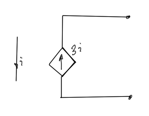
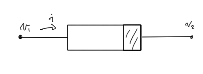
    Imagine, for example, that we have a component illustrated in fig. 1.

    fig. 1.  Variable voltage device

    fig. 1. Variable voltage device

    \begin{equation}\label{eqn:multiphysicsL4:20}
    v_1 – v_2 = 3 i^2
    \end{equation}

  • any current which is controlling dependent sources, as in fig. 2.
    fig. 2.  Current controlled device

    fig. 2. Current controlled device

  • Inductors
    \begin{equation}\label{eqn:multiphysicsL4:40}
    v_1 – v_2 = L \frac{di}{dt}.
    \end{equation}

Solving large systems

We are interested in solving linear systems of the form

\begin{equation}\label{eqn:multiphysicsL4:60}
M \overline{{x}} = \overline{{b}},
\end{equation}

possibly with thousands of elements.

Gaussian elimination

\begin{equation}\label{eqn:multiphysicsL4:80}
\begin{bmatrix}
M_{11} & M_{12} & M_{13} \\
M_{21} & M_{22} & M_{23} \\
M_{31} & M_{32} & M_{33} \\
\end{bmatrix}
\begin{bmatrix}
x_1 \\
x_2 \\
x_3 \\
\end{bmatrix}
=
\begin{bmatrix}
b_1 \\
b_2 \\
b_3 \\
\end{bmatrix}
\end{equation}

It’s claimed for now, to be seen later, that back substitution is the fastest way to arrive at the solution, less computationally complex than completion the diagonalization.

Steps

\begin{equation}\label{eqn:multiphysicsL4:100}
(1) \cdot \frac{M_{21}}{M_{11}} \Rightarrow
\begin{bmatrix}
M_{21} & \frac{M_{21}}{M_{11}} M_{12} & \frac{M_{21}}{M_{11}} M_{13} \\
\end{bmatrix}
\end{equation}

\begin{equation}\label{eqn:multiphysicsL4:120}
(2) \cdot \frac{M_{31}}{M_{11}} \Rightarrow
\begin{bmatrix}
M_{31} & \frac{M_{31}}{M_{11}} M_{32} & \frac{M_{31}}{M_{11}} M_{33} \\
\end{bmatrix}
\end{equation}

This gives

\begin{equation}\label{eqn:multiphysicsL4:140}
\begin{bmatrix}
M_{11} & M_{12} & M_{13} \\
0 & M_{22} – \frac{M_{21}}{ M_{11} } M_{12} & M_{23} – \frac{M_{21}}{M_{11}} M_{13} \\
0 & M_{32} – \frac{M_{31}}{M_{11}} M_{32} & M_{33} – \frac{M_{31}}{M_{11}} M_{33} \\
\end{bmatrix}
\begin{bmatrix}
x_1 \\
x_2 \\
x_3 \\
\end{bmatrix}
=
\begin{bmatrix}
b_1 \\
b_2 – \frac{M_{21}}{M_{11}} b_1 \\
b_3 – \frac{M_{31}}{M_{11}} b_1
\end{bmatrix}.
\end{equation}

Here the \( M_{11} \) element is called the {pivot}. Each of the \(
M_{j1}/M_{11} \) elements is called a {multiplier}. This operation can be written as

\begin{equation}\label{eqn:multiphysicsL4:160}
\begin{bmatrix}
M_{11} & M_{12} & M_{13} \\
0 & M_{22}^{(2)} & M_{23}^{(3)} \\
0 & M_{32}^{(2)} & M_{33}^{(3)} \\
\end{bmatrix}
\begin{bmatrix}
x_1 \\
x_2 \\
x_3 \\
\end{bmatrix}
=
\begin{bmatrix}
b_1 \\
b_2^{(2)} \\
b_3^{(2)} \\
\end{bmatrix}.
\end{equation}

Using \( M_{22}^{(2)} \) as the pivot this time, we form
\begin{equation}\label{eqn:multiphysicsL4:180}
\begin{bmatrix}
M_{11} & M_{12} & M_{13} \\
0 & M_{22}^{(2)} & M_{23}^{(3)} \\
0 & 0 & M_{33}^{(3)} – \frac{M_{32}^{(2)}}{M_{22}^{(2)}} M_{23}^{(2)} \\
\end{bmatrix}
\begin{bmatrix}
x_1 \\
x_2 \\
x_3 \\
\end{bmatrix}
=
\begin{bmatrix}
b_1 \\
b_2 – \frac{M_{21}}{M_{11}} b_1 \\
b_3 – \frac{M_{31}}{M_{11}} b_1
– \frac{M_{32}^{(2)}}{M_{22}^{(2)}} b_{2}^{(2)} \\
\end{bmatrix}.
\end{equation}

LU decomposition

Through Gaussian elimination, we have transformed the system from

\begin{equation}\label{eqn:multiphysicsL4:200}
M x = b
\end{equation}

to
\begin{equation}\label{eqn:multiphysicsL4:220}
U x = y.
\end{equation}

Writing out our Gaussian transformation in the form \( U \overline{{x}} = b \) we have

\begin{equation}\label{eqn:multiphysicsL4:240}
U \overline{{x}} =
\begin{bmatrix}
1 & 0 & 0 \\
-\frac{M_{21}}{M_{11}} & 1 & 0 \\
\frac{M_{32}^{(2)}}{M_{22}^{(2)}}
\frac{M_{21}}{M_{11}}

\frac{M_{31}}{M_{11}}
&

\frac{M_{32}^{(2)}}{M_{22}^{(2)}}
& 1
\end{bmatrix}
\begin{bmatrix}
b_1 \\
b_2 \\
b_3
\end{bmatrix}.
\end{equation}

We can verify that the operation matrix \( K^{-1} \), where \( K^{-1} U = M \) that takes us to this form is

\begin{equation}\label{eqn:multiphysicsL4:260}
\begin{bmatrix}
1 & 0 & 0 \\
\frac{M_{21}}{M_{11}} & 1 & 0 \\
\frac{M_{31}}{M_{11}} &
\frac{M_{32}^{(2)}}{M_{22}^{(2)}} &
1
\end{bmatrix}
\begin{bmatrix}
U_{11} & U_{12} & U_{13} \\
0 & U_{22} & U_{23} \\
0 & 0 & U_{33} \\
\end{bmatrix}
\overline{{x}} = \overline{{b}}
\end{equation}

Using this {LU} decomposition is generally superior to standard Gaussian elimination, since we can use this for many different \(\overline{{b}}\) vectors using the same amount of work.

Our steps are

\begin{equation}\label{eqn:multiphysicsL4:280}
b
= M x
= L \lr{ U x}
\equiv L y.
\end{equation}

We can now solve \( L y = b \), using substitution for \( y_1 \), then \( y_2 \), and finally \( y_3 \). This is called {forward substitution}.

Finally, we can now solve

\begin{equation}\label{eqn:multiphysicsL4:300}
U x = y,
\end{equation}

using {back substitution}.

Note that we produced the vector \( y \) as a side effect of performing the Gaussian elimination process.

It is already time for remembrance day propaganda

September 24, 2014 Incoherent ramblings , , , ,


The propaganda for celebration of war, destruction, killing, and rape is already starting.  I was greeted today on facebook by the serene and smiling image of a world war II vet, along with his seemingly innocent request for “likes”

10685554_10152729206678582_3200916120344147288_n

This is probably supposed to make people feel patriotism, the worship of an artificial boundary on a map and its associated label system.  Patriotism and national pride worship are designed to ensure that no rational thought opposes the psychopathic figureheads that run our modern “democracies”.

When we see vet worship propaganda like this, you have to think about the interests that encouraged the war in the first place.  These are power brokers like the Carnegies that requested that Wilson not end the war (WWI) too soon (and who had concluded in their minutes before that there was no better institution for profits than the business of war).  These are the armaments and munitions  manufacturers.  These are the companies that built the tanks and the planes that bombed uncounted civilians in Germany and the UK.  These are the makers of weapons that use white phosphorus and depleted uranium, and the makers of cluster bombs that shred children into hamburger meat before and after they are deployed.

I would describe us as being in world war III now.  This is the series of undeclared and covert wars that the USA and NATO have waged since world war II.  This is a war that happens with our tacit approval.  This approval that is assumed because there is no widespread disapproval.  Unfortunately, so much of this modern and current war happens without our even knowing about it, that nobody thinks to object.  This war is disconnected from our immediate attention, and most of the time we don’t even realize that we are funding it.  As always, I don’t want my tax dollars, money stolen from me at the point of a gun, to be used to fund the slaughter of people in Yugoslavia or Libya or <enter your favorite target in some little known corner of the world>, but I can’t control this.  It happens again and again, and is truly disgusting.

I am happy to see that this poor fellow survived.  However, if he had fought a real war, it would have been the war against the propaganda and brainwashing that involved him in the combat that got most of his compatriots killed, and against the same combat that killed uncountable numbers of civilians and “enemies”, and against the combat that encouraged these “enemies” to do the same.

I will not be liking this picture.

ECE1254H Modeling of Multiphysics Systems. Lecture 3: Nodal Analysis. Taught by Prof. Piero Triverio

September 24, 2014 ece1254 , , ,

[Click here for a PDF of this post with nicer formatting]

Disclaimer

Peeter’s lecture notes from class. These may be incoherent and rough.

Nodal Analysis

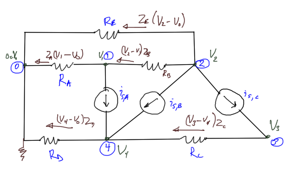
Avoiding branch currents can reduce the scope of the computational problem. Consider the same circuit fig. 1, this time introducing only node voltages as unknowns

fig. 1.  Resistive circuit with current sources

fig. 1. Resistive circuit with current sources

Unknowns: node voltages: \(V_1, V_2, \cdots V_4\)

Equations are KCL at each node except \(0\).

  1. \(
    \frac{V_1 – 0}{R_A} +
    \frac{V_1 – V_2}{R_B} + i_{S,A} = 0
    \)

  2. \(
    \frac{V_2 – 0}{R_E} +
    \frac{V_2 – V_1}{R_B} + i_{S,B} + i_{S,C} = 0
    \)

  3. \(
    \frac{V_3 – V_4}{R_C} – i_{S,C} = 0
    \)

  4. \(
    \frac{V_4 – 0}{R_D}
    +\frac{V_4 – V_3}{R_C}
    – i_{S,A} – i_{S,B} = 0
    \)

In matrix form this is

\begin{equation}\label{eqn:multiphysicsL3:20}
\begin{bmatrix}
\inv{R_A} + \inv{R_B} & – \inv{R_B} & 0 & 0 \\
-\inv{R_B} & \inv{R_B} + \inv{R_E} & 0 & 0 \\
0 & 0 & \inv{R_C} & -\inv{R_C} \\
0 & 0 & -\inv{R_C} & \inv{R_C} + \inv{R_D}
\end{bmatrix}
\begin{bmatrix}
V_1 \\
V_2 \\
V_3 \\
V_4 \\
\end{bmatrix}
=
\begin{bmatrix}
-i_{S,A} \\
-i_{S,B} – i_{S,C} \\
i_{S,C} \\
i_{S,A} + i_{S,B}
\end{bmatrix}
\end{equation}

Introducing the nodal matrix

\begin{equation}\label{eqn:multiphysicsL3:40}
G \overline{{V}}_N = \overline{{I}}_S
\end{equation}

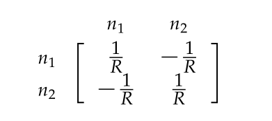
We identify the {stamp} for a resister of value \(R\) between nodes \(n_1\) and \(n_2\)

stamp matrix

stamp matrix

where we have a set of rows and columns for each of the node voltages \(n_1, n_2\).

Note that some care is required to use this nodal analysis method since we required the invertible relationship \(i = V/R\). We also cannot handle short circuits \(V = 0\), or voltage sources \(V = 5\) (say). We will also have trouble with differential terms like inductors.

Recap of node branch equations

We had

  • KCL: \( A \cdot \overline{{I}}_B = \overline{{I}}_S\)
  • Constitutive: \( \overline{{I}}_B = \alpha A^\T \overline{{V}}_N \),
  • Nodal equations: \( A \alpha A^\T \overline{{V}}_N = \overline{{I}}_S \)

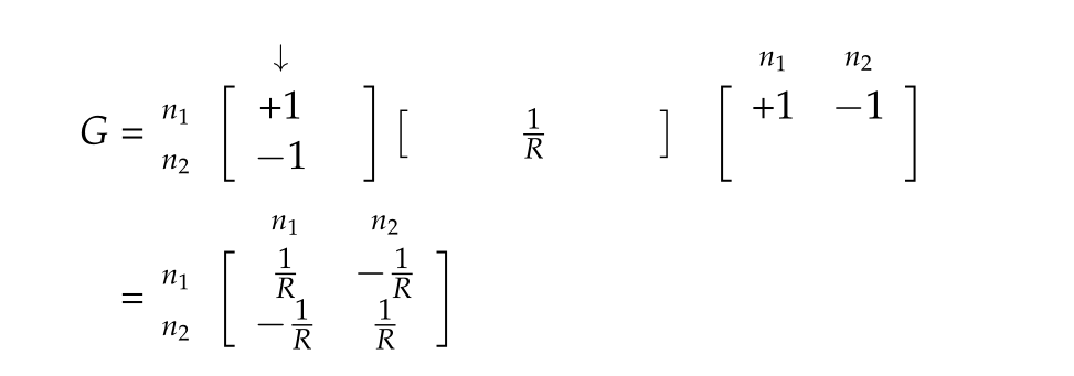
where \(\overline{{I}}_B\) was the branch currents, \(A\) was the incidence matrix, and \(\alpha = \begin{bmatrix}\inv{R_1} & & \\ & \inv{R_2} & \\ & & \ddots \end{bmatrix} \).

The stamp can be observed in the multiplication of the contribution for a single resistor, where we see that the incidence matrix has the form \( G = A \alpha A^\T \)

stamp factor

stamp factor

Theoretical facts

Noting that \(\lr{ A B }^\T = B^\T A^\T \), it is clear that the nodal matrix \(G = A \alpha A^\T \) is symmetric

\begin{equation}\label{eqn:multiphysicsL3:80}
G^\T
=
\lr{ A \alpha A^\T }^\T
=
\lr{ A^\T }^\T \alpha^\T A^\T
=
A \alpha A^\T
= G
\end{equation}

Modified nodal analysis (MNA)

This is the method that we find in software such as spice.

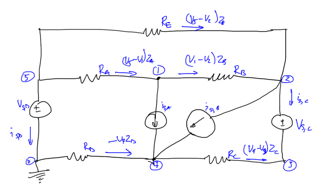
To illustrate the method, consider the same circuit, augmented with an additional voltage sources as in fig. 4.

fig. 4.  Resistive circuit with current and voltage sources

fig. 4. Resistive circuit with current and voltage sources

We know wish to have the following unknowns

  • node voltages (\(N-1\)): \( V_1, V_2, \cdots V_5 \)
  • branch currents for selected components (\(K\)): \( i_{S,C}, i_{S,D} \)

We will have two less unknowns for this system than with standard nodal analysis. Our equations are

  1. \(
    -\frac{V_5-V_1}{R_A}
    +\frac{V_1-V_2}{R_B}
    + i_{S,A} = 0
    \)

  2. \(
    \frac{V_2-V_5}{R_E}
    +\frac{V_2-V_1}{R_B}
    + i_{S,B}
    + i_{S,C}
    = 0
    \)

  3. \(
    -i_{S,C} +
    \frac{V_3-V_4}{R_C} = 0
    \)

  4. \(
    \frac{V_4-0}{R_D}
    +\frac{V_4-V_3}{R_C}
    – i_{S,A}
    – i_{S,B}
    = 0
    \)

  5. \(
    \frac{V_5-V_2}{R_E}
    +\frac{V_5-V_1}{R_A}
    + i_{S,D} = 0
    \)

Put into giant matrix form, this is

giant matrix

giant matrix

Call the extension to the nodal matrix \(G\), the {voltage incidence matrix} \(A_V\).