Square of electrodynamic field.

June 5, 2022 math and physics play , , , , ,

[Click here for a PDF version of this post]

The electrodynamic Lagrangian (without magnetic sources) has the form
\begin{equation}\label{eqn:fsquared:20}
\LL = F \cdot F + \alpha A \cdot J,
\end{equation}
where \( \alpha \) is a constant that depends on the unit system.
My suspicion is that one or both of the bivector or quadvector grades of \( F^2 \) are required for Maxwell’s equation with magnetic sources.

Let’s expand out \( F^2 \) in coordinates, as preparation for computing the Euler-Lagrange equations. The scalar and pseudoscalar components both simplify easily into compact relationships, but the bivector term is messier. We start with the coordinate expansion of our field, which we may write in either upper or lower index form
\begin{equation}\label{eqn:fsquared:40}
F = \inv{2} \gamma_\mu \wedge \gamma_\nu F^{\mu\nu}
= \inv{2} \gamma^\mu \wedge \gamma^\nu F_{\mu\nu}.
\end{equation}
The square is
\begin{equation}\label{eqn:fsquared:60}
F^2 = F \cdot F + \gpgradetwo{F^2} + F \wedge F.
\end{equation}

Let’s compute the scalar term first. We need to make a change of dummy indexes, for one of the \( F \)’s. It will also be convenient to use upper indexes in one factor, and lowers in the other. We find
\begin{equation}\label{eqn:fsquared:80}
\begin{aligned}
F \cdot F
&=
\inv{4}
\lr{ \gamma_\mu \wedge \gamma_\nu } \cdot \lr{ \gamma^\alpha \wedge \gamma^\beta }
F^{\mu\nu}
F_{\alpha\beta} \\
&=
\inv{4}
\lr{
{\delta_\nu}^\alpha {\delta_\mu}^\beta
– {\delta_\mu}^\alpha {\delta_\nu}^\beta
}
F^{\mu\nu}
F_{\alpha\beta} \\
&=
\inv{4}
\lr{
F^{\mu\nu} F_{\nu\mu}

F^{\mu\nu} F_{\mu\nu}
} \\
&=
-\inv{2}
F^{\mu\nu} F_{\mu\nu}.
\end{aligned}
\end{equation}

Now, let’s compute the pseudoscalar component of \( F^2 \). This time we uniformly use upper index components for the tensor, and find
\begin{equation}\label{eqn:fsquared:100}
\begin{aligned}
F \wedge F
&=
\inv{4}
\lr{ \gamma_\mu \wedge \gamma_\nu } \wedge \lr{ \gamma_\alpha \wedge \gamma_\beta }
F^{\mu\nu}
F^{\alpha\beta} \\
&=
\frac{I}{4}
\epsilon_{\mu\nu\alpha\beta} F^{\mu\nu} F^{\alpha\beta},
\end{aligned}
\end{equation}
where \( \epsilon_{\mu\nu\alpha\beta} \) is the completely antisymmetric (Levi-Civita) tensor of rank four. This pseudoscalar components picks up all the products of components of \( F \) where all indexes are different.

Now, let’s try computing the bivector term of the product. This will require fancier index gymnastics.
\begin{equation}\label{eqn:fsquared:120}
\begin{aligned}
\gpgradetwo{F^2}
&=
\inv{4}
\gpgradetwo{
\lr{ \gamma_\mu \wedge \gamma_\nu } \lr{ \gamma^\alpha \wedge \gamma^\beta }
}
F^{\mu\nu}
F_{\alpha\beta} \\
&=
\inv{4}
\gpgradetwo{
\gamma_\mu \gamma_\nu \lr{ \gamma^\alpha \wedge \gamma^\beta }
}
F^{\mu\nu}
F_{\alpha\beta}

\inv{4}
\lr{ \gamma_\mu \cdot \gamma_\nu} \lr{ \gamma^\alpha \wedge \gamma^\beta } F^{\mu\nu} F_{\alpha\beta}.
\end{aligned}
\end{equation}
The dot product term is killed, since \( \lr{ \gamma_\mu \cdot \gamma_\nu} F^{\mu\nu} = g_{\mu\nu} F^{\mu\nu} \) is the contraction of a symmetric tensor with an antisymmetric tensor. We can now proceed to expand the grade two selection
\begin{equation}\label{eqn:fsquared:140}
\begin{aligned}
\gpgradetwo{
\gamma_\mu \gamma_\nu \lr{ \gamma^\alpha \wedge \gamma^\beta }
}
&=
\gamma_\mu \wedge \lr{ \gamma_\nu \cdot \lr{ \gamma^\alpha \wedge \gamma^\beta } }
+
\gamma_\mu \cdot \lr{ \gamma_\nu \wedge \lr{ \gamma^\alpha \wedge \gamma^\beta } } \\
&=
\gamma_\mu \wedge
\lr{
{\delta_\nu}^\alpha \gamma^\beta

{\delta_\nu}^\beta \gamma^\alpha
}
+
g_{\mu\nu} \lr{ \gamma^\alpha \wedge \gamma^\beta }

{\delta_\mu}^\alpha \lr{ \gamma_\nu \wedge \gamma^\beta }
+
{\delta_\mu}^\beta \lr{ \gamma_\nu \wedge \gamma^\alpha } \\
&=
{\delta_\nu}^\alpha \lr{ \gamma_\mu \wedge \gamma^\beta }

{\delta_\nu}^\beta \lr{ \gamma_\mu \wedge \gamma^\alpha }

{\delta_\mu}^\alpha \lr{ \gamma_\nu \wedge \gamma^\beta }
+
{\delta_\mu}^\beta \lr{ \gamma_\nu \wedge \gamma^\alpha }.
\end{aligned}
\end{equation}
Observe that I’ve taken the liberty to drop the \( g_{\mu\nu} \) term. Strictly speaking, this violated the equality, but won’t matter since we will contract this with \( F^{\mu\nu} \). We are left with
\begin{equation}\label{eqn:fsquared:160}
\begin{aligned}
4 \gpgradetwo{ F^2 }
&=
\lr{
{\delta_\nu}^\alpha \lr{ \gamma_\mu \wedge \gamma^\beta }

{\delta_\nu}^\beta \lr{ \gamma_\mu \wedge \gamma^\alpha }

{\delta_\mu}^\alpha \lr{ \gamma_\nu \wedge \gamma^\beta }
+
{\delta_\mu}^\beta \lr{ \gamma_\nu \wedge \gamma^\alpha }
}
F^{\mu\nu}
F_{\alpha\beta} \\
&=
F^{\mu\nu}
\lr{
\lr{ \gamma_\mu \wedge \gamma^\alpha }
F_{\nu\alpha}

\lr{ \gamma_\mu \wedge \gamma^\alpha }
F_{\alpha\nu}

\lr{ \gamma_\nu \wedge \gamma^\alpha }
F_{\mu\alpha}
+
\lr{ \gamma_\nu \wedge \gamma^\alpha }
F_{\alpha\mu}
} \\
&=
2 F^{\mu\nu}
\lr{
\lr{ \gamma_\mu \wedge \gamma^\alpha }
F_{\nu\alpha}
+
\lr{ \gamma_\nu \wedge \gamma^\alpha }
F_{\alpha\mu}
} \\
&=
2 F^{\nu\mu}
\lr{ \gamma_\nu \wedge \gamma^\alpha }
F_{\mu\alpha}
+
2 F^{\mu\nu}
\lr{ \gamma_\nu \wedge \gamma^\alpha }
F_{\alpha\mu},
\end{aligned}
\end{equation}
which leaves us with
\begin{equation}\label{eqn:fsquared:180}
\gpgradetwo{ F^2 }
=
\lr{ \gamma_\nu \wedge \gamma^\alpha }
F^{\mu\nu}
F_{\alpha\mu}.
\end{equation}
I suspect that there must be an easier way to find this result.

We now have the complete coordinate expansion of \( F^2 \), separated by grade
\begin{equation}\label{eqn:fsquared:200}
F^2 =
-\inv{2}
F^{\mu\nu} F_{\mu\nu}
+
\lr{ \gamma_\nu \wedge \gamma^\alpha }
F^{\mu\nu}
F_{\alpha\mu}
+
\frac{I}{4}
\epsilon_{\mu\nu\alpha\beta} F^{\mu\nu} F^{\alpha\beta}.
\end{equation}
Tomorrow’s task is to start evaluating the Euler-Lagrange equations for this multivector Lagrangian density, and see what we get.

Almost an academic author: Appendix B: Representation of Dyadics via Geometric Algebra

May 29, 2022 math and physics play , , ,

I corresponded for a bit with the author of a paper on variations and inconsistencies with dyadic notation that is used in some fluid flow and other problems.  In the end I ended up contributing an appendix (Appendix B: Representation of Dyadics via Geometric Algebra) to their paper, which has been submitted to an academic journal (I forget which one.)

I’ve written thousands of pages of independent musings as blog posts, and even a book (self published, and also available for free in pdf form), but this is the first time anything that I’ve written has ended up in an academic journal.

You can find a preprint here on arxiv

New revision of my book: Geometric Algebra for Electrical Engineers

May 16, 2022 Geometric Algebra for Electrical Engineers

A new version of my book is now available in free pdf form, in paperback and hardcover on amazon, on leanpub, and for the brave or crazy — as latex source files and a makefile.  All of these can be found here:

Geometric Algebra for Electrical Engineers.


Changes in this V0.1.16-13 (May 15, 2022) version, include:

  • Fix equations 2.81 2.82 — error found by Christopher
  • test drove build instructions (slight fix required.)
  • restore latexsym \Box as dAlembertian
  • gutter fixes.
  • perl -p -i -e ‘s/ *$//’ `cat spellcheckem.txt `
  • (massive change with no visible effects if done right): purge most dmath usage. MacTex upgrade has made these seemingly malfunction, and lines are getting split in all sorts of weird places.

The C compiler is too forgiving! sizeof(variable_name+1) allowed?

April 28, 2022 C/C++ development and debugging. , , , ,

I carelessly passed:

sizeof(s.st_size+1)

to an allocator call, instead of:

s.st_size+1

and corrupted memory nicely.

What the hell would sizeof(variable+1) even mean, and why on earth would the compiler think that is anything close to valid? Both gcc and clang, each with -Wall, are completely quiet about this error!

Curvilinear coordinates and reciprocal frames.

April 5, 2022 math and physics play

[Click here for a PDF version of this post]

Curvilinear coordinates.

Let’s start by considering a two parameter surface specified by \( \Bx = \Bx(a,b) \). This defines a surface, for which the partials are both tangent to at each point of the surface. We write
\begin{equation}\label{eqn:reciprocalAndTangentspace:20}
\begin{aligned}
\Bx_a &= \PD{a}{\Bx} \\
\Bx_b &= \PD{b}{\Bx}.
\end{aligned}
\end{equation}
We call \( \text{span}\setlr{ \Bx_a, \Bx_b } \) the tangent space of the surface at the parameter values \( a,b \). One important role of the curvilinear vectors \( \Bx_a, \Bx_b \) is to describe the area element for the subspace
\begin{equation}\label{eqn:reciprocalAndTangentspace:40}
d\Bx_a \wedge d\Bx_b
=
\lr{ \Bx_a \wedge \Bx_b } da db.
\end{equation}
Observe that for a two dimensional space, this has the form
\begin{equation}\label{eqn:reciprocalAndTangentspace:60}
d\Bx_a \wedge d\Bx_b =
\begin{vmatrix}
\Bx_a & \Bx_b
\end{vmatrix} \Bi\, da db,
\end{equation}
where \( \Bi \) is the pseudoscalar for the space. The reader may be familiar with the determinant here, which is the Jacobian encountered in a change of variable context. We may generalize this idea of tangent space to more variables in an obvious fashion. For example, given
\begin{equation}\label{eqn:reciprocalAndTangentspace:80}
\Bx = \Bx(a^1, a^2, \cdots, a^M),
\end{equation}
we write
\begin{equation}\label{eqn:reciprocalAndTangentspace:100}
\Bx_{a^i} = \PD{a^i}{\Bx}.
\end{equation}

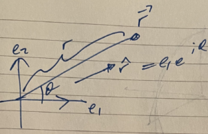
Let’s look at some examples, starting with circular coordinates in a plane
\begin{equation}\label{eqn:reciprocalAndTangentspace:120}
\Bx(r, \theta) = r \Be_1 e^{i\theta},
\end{equation}
where \( i = \Be_1 \Be_2 \). Our tangent space vectors are
\begin{equation}\label{eqn:reciprocalAndTangentspace:140}
\Bx_r = \Be_1 e^{i\theta},
\end{equation}
and
\begin{equation}\label{eqn:reciprocalAndTangentspace:160}
\Bx_\theta
= r \Be_1 i e^{i\theta}
= r \Be_2 e^{i\theta}.
\end{equation}
The area element in this case is
\begin{equation}\label{eqn:reciprocalAndTangentspace:180}
d\Bx_r \wedge d\Bx_\theta
=
\Bx_r \wedge \Bx_\theta dr d\theta
=
\gpgradetwo{
\Be_1 e^{i\theta}
r \Be_2 e^{i\theta} }
dr d\theta
= i r dr d\theta.
\end{equation}
Integration over a circular region gives
\begin{equation}\label{eqn:reciprocalAndTangentspace:200}
\int_{r = 0}^R \int_{\theta=0}^{2\pi} d\Bx_r \wedge d\Bx_\theta
=
i \int_{r = 0}^R
r dr
\int_{\theta=0}^{2\pi}
d\theta
=
i \frac{R^2}{2} 2 \pi
= i \pi R^2.
\end{equation}
This is the area of the circle, scaled by the unit bivector that represents the orientation of the plane in this two dimensional subspace.

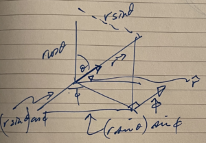
As another example, consider a spherical parameterization, as illustrated in fig. 1.
\begin{equation}\label{eqn:reciprocalAndTangentspace:220}
\Bx(r, \theta, \phi) = r \Be_1 e^{i\phi} \sin\theta + r \Be_3 \cos\theta.
\end{equation}

fig. 1. Spherical coordinates.

Our curvilinear vectors in this case are
\begin{equation}\label{eqn:reciprocalAndTangentspace:240}
\Bx_r = \Be_1 e^{i\phi} \sin\theta + \Be_3 \cos\theta,
\end{equation}
\begin{equation}\label{eqn:reciprocalAndTangentspace:260}
\Bx_\theta = r \Be_1 e^{i\phi} \cos\theta – r \Be_3 \sin\theta,
\end{equation}
\begin{equation}\label{eqn:reciprocalAndTangentspace:280}
\Bx_\phi = r \Be_2 e^{i\phi} \sin\theta.
\end{equation}
In this case our (pseudoscalar) volume element is
\begin{equation}\label{eqn:reciprocalAndTangentspace:300}
\begin{aligned}
d\Bx_r \wedge
d\Bx_\theta \wedge
d\Bx_\phi
&=
r^2 \sin\theta \gpgradethree{
\lr{ \Be_1 e^{i\phi} \sin\theta + \Be_3 \cos\theta }
\lr{ \Be_1 e^{i\phi} \cos\theta – \Be_3 \sin\theta }
\Be_2 e^{i\phi}
}
\, dr d\theta d\phi \\
&=
r^2 \sin\theta \gpgradethree{
\lr{ \Be_1 e^{i\phi} \sin\theta + \Be_3 \cos\theta }
\lr{ \Be_1 \cos\theta – \Be_3 e^{-i\phi} \sin\theta }
\Be_2
} \, dr d\theta d\phi \\
&=
r^2 \sin\theta \gpgradethree{
\lr{ -\Be_1 \Be_3 \sin^2\theta
+
\Be_3 \Be_1 \cos^2\theta
}
\Be_2
} \, dr d\theta d\phi \\
&=
\Be_3 \Be_1 \Be_2 r^2 \sin\theta
\, dr d\theta d\phi \\
&=
I r^2 \sin \theta
\, dr d\theta d\phi.
\end{aligned}
\end{equation}
This is just the standard spherical volume element, but scaled with the pseudoscalar. If we integrate the upper half of the volume (above the x-y plane), we would find \( \int_{r=0}^R \int_{\phi=0}^{2 \pi} \int_{\theta=0}^{\pi/2} d\Bx_r \wedge d\Bx_\theta \wedge d\Bx_\phi = (1/2) I (4/3) \pi R^3 \), half the volume of the sphere, again weighted by the pseudoscalar for the space. The sign would be negated for the lower half of plane, since our volume element is not strictly positive everywhere. This change of sign is not unique to this geometric algebra formulation, as we would have to integrate \( \int \Abs{\partial(x, y, z)/\partial(r,\theta, \phi)} \, dr d\theta d\phi \) if we were computing the spherical volume using a standard scalar change of variables (taking the absolute value of our Jacobian.)

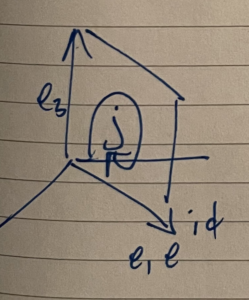
As a final example, let’s pick the coordinates associated with a relativistic boost and scale parameterization in spacetime, illustrated in fig. 2, with \( r = 1 \).

fig. 2. Boost worldline.

\begin{equation}\label{eqn:reciprocalAndTangentspace:360}
x = r \gamma_0 e^{\gamma_0 \gamma_1 \alpha}.
\end{equation}
For this surface we have
\begin{equation}\label{eqn:reciprocalAndTangentspace:380}
\begin{aligned}
x_r &= \gamma_0 e^{\gamma_0 \gamma_1 \alpha} \\
x_\alpha &= r \gamma_1 e^{\gamma_0 \gamma_1 \alpha}.
\end{aligned}
\end{equation}
In this case the volume element is
\begin{equation}\label{eqn:reciprocalAndTangentspace:400}
dx_r \wedge dx_\alpha
= r dr d\alpha \gpgradetwo{
\gamma_0 e^{\gamma_{01} \alpha}
\gamma_1 e^{\gamma_{01} \alpha}
}
= r dr d\alpha \gpgradetwo{
\gamma_0
\gamma_1
e^{-\gamma_{01} \alpha}
e^{\gamma_{01} \alpha}
}
= \gamma_{01} r dr d\alpha.
\end{equation}
This is cosmetically similar to the circular area element above, also weighted by a pseudoscalar, but in this case, \( \alpha \) is not restricted to a bounded interval. We also see that the basic ideas here work for both Euclidean and non-Euclidean vector spaces.

Reciprocal frame vectors.

Returning to a two dimensional surface, with tangent plane \( \text{span}\setlr{ \Bx_a, \Bx_b } \), any vector in that plane has the form
\begin{equation}\label{eqn:reciprocalAndTangentspace:320}
\By = y^a \Bx_a + y^b \Bx_b.
\end{equation}
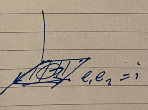
This is illustrated in fig. 3.

fig. 3. Tangent plane for two parameter surface.

Coordinates.

We call \( y^a, y^b \) the coordinates of the vector \( \By \) with respect to the basis for the tangent space \( \text{span}\setlr{ \Bx_a, \Bx_b } \). The computation of these coordinates is facilitated by finding the reciprocal frame \( \Bx^a, \Bx^b \) for the tangent space that satisfies both \( \Bx^a, \Bx^b \in \text{span} \setlr{\Bx_a, \Bx_b } \), and
\begin{equation}\label{eqn:reciprocalAndTangentspace:340}
\Bx^\mu \cdot \Bx_\nu = {\delta^\mu}_\nu,
\end{equation}
for all \( \mu \in \setlr{a,b} \).

We may demonstrate that this works by example, dotting with each of our reciprocal frame vectors
\begin{equation}\label{eqn:reciprocalAndTangentspace:420}
\begin{aligned}
y \cdot \Bx^a
&=
\lr{ y^a \Bx_a + y^b \Bx_b } \cdot \Bx^a \\
&=
y^a \lr{ \Bx_a \cdot \Bx^a } + y^b \lr{\Bx_b \cdot \Bx^a } \\
&= y^a,
\end{aligned}
\end{equation}
and similarly
\begin{equation}\label{eqn:reciprocalAndTangentspace:440}
\begin{aligned}
y \cdot \Bx^b
&=
\lr{ y^a \Bx_a + y^b \Bx_b } \cdot \Bx^b \\
&=
y^a \lr{ \Bx_a \cdot \Bx^b } + y^b \lr{\Bx_b \cdot \Bx^b } \\
&= y^b.
\end{aligned}
\end{equation}
Provided we can find these reciprocal vectors, they provide the projections along each of the respective directions, allowing us to formulate the coordinate decomposition with respect to either the curvilinear or the reciprocal basis
\begin{equation}\label{eqn:reciprocalAndTangentspace:460}
\By =
\lr{ \By \cdot \Bx^a } \Bx_a
+
\lr{ \By \cdot \Bx^b } \Bx_b
=
\lr{ \By \cdot \Bx_a } \Bx^a
+
\lr{ \By \cdot \Bx_b } \Bx^b.
\end{equation}
For orthonornal Euclidean vectors, this reduces to the familiar sum of projections

\begin{equation}\label{eqn:reciprocalAndTangentspace:480}
\Bx = \sum_i \lr{ \Bx \cdot \Be_i } \Be_i.
\end{equation}
The reciprocal frame allows us to find the coordinates with respect to a oblique (non-orthonormal) basis, also not imposing a requirement for the space to be Euclidean.

Orthogonal curvilinear coordinates.

When our tangent plane vectors are orthogonal, computation of the reciprocal frame just requires scaling. That scaling, perhaps not suprisingly, given the name reciprocal, just requires a vector inverse. For our two parameter case, that is just
\begin{equation}\label{eqn:reciprocalAndTangentspace:500}
\Bx^a = \inv{\Bx_a} = \frac{\Bx_a}{\Bx_a \cdot \Bx_a}
, \quad
\Bx^b = \inv{\Bx_b} = \frac{\Bx_b}{\Bx_b \cdot \Bx_b}.
\end{equation}
The reader can readily verify that \( \Bx^a \cdot \Bx_a = \Bx^b \cdot \Bx_b = 1 \), and \( \Bx^a \cdot \Bx_b = \Bx^b \cdot \Bx_a = 0 \).

As an example, using the circular frame considered above, where we had
\begin{equation}\label{eqn:reciprocalAndTangentspace:520}
\begin{aligned}
\Bx_r &= \Be_1 e^{i\theta} \\
\Bx_\theta &= r \Be_2 e^{i\theta},
\end{aligned}
\end{equation}
the reciprocals are just
\begin{equation}\label{eqn:reciprocalAndTangentspace:540}
\begin{aligned}
\Bx^r &= \Be_1 e^{i\theta} \\
\Bx^\theta &= \inv{r} \Be_2 e^{i\theta}.
\end{aligned}
\end{equation}
In this specific case, the reader can also readily verify that \( \Bx^r \cdot \Bx_r = \Bx^\theta \cdot \Bx_\theta = 1 \), and \( \Bx^r \cdot \Bx_\theta = \Bx^\theta \cdot \Bx_r = 0 \).

Similarly, for the spherical frame basis (\ref{eqn:reciprocalAndTangentspace:240}, …), we have
\begin{equation}\label{eqn:reciprocalAndTangentspace:560}
\Bx_r^2 = \Abs{e^{i\phi} \sin\theta}^2 + \cos^2\theta = 1,
\end{equation}
\begin{equation}\label{eqn:reciprocalAndTangentspace:580}
\Bx_\theta^2 = r^2 \lr{ \Abs{e^{i\phi} \cos\theta}^2 + \sin^2\theta } = r^2,
\end{equation}
and
\begin{equation}\label{eqn:reciprocalAndTangentspace:600}
\Bx_\phi^2 = r^2 \sin^2\theta,
\end{equation}
so the spherical reciprocals are just
\begin{equation}\label{eqn:reciprocalAndTangentspace:620}
\Bx^r = \Be_1 e^{i\phi} \sin\theta + \Be_3 \cos\theta,
\end{equation}
\begin{equation}\label{eqn:reciprocalAndTangentspace:640}
\Bx^\theta = \inv{r} \lr{ \Be_1 e^{i\phi} \cos\theta – \Be_3 \sin\theta},
\end{equation}
\begin{equation}\label{eqn:reciprocalAndTangentspace:660}
\Bx^\phi = \inv{r \sin\theta} \Be_2 e^{i\phi}.
\end{equation}

Using straight inversion to compute the reciprocal frame vectors even works for non-Euclidean spaces. Consider the following example, using the relativisitic (Dirac) basis
\begin{equation}\label{eqn:reciprocalAndTangentspace:680}
x(a,b) = a \lr{ \gamma_1 + \gamma_2 } + b \gamma_3,
\end{equation}
for which we have
\begin{equation}\label{eqn:reciprocalAndTangentspace:700}
x_a = \gamma_1 + \gamma_2,
\end{equation}
and
\begin{equation}\label{eqn:reciprocalAndTangentspace:720}
x_b = \gamma_3.
\end{equation}
We have to be a bit more careful to compute the squares for this mixed metric space, but if we do that, we find
\begin{equation}\label{eqn:reciprocalAndTangentspace:740}
x_a^2 =
\gamma_1^2 + \gamma_2^2
= -2,
\end{equation}
and
\begin{equation}\label{eqn:reciprocalAndTangentspace:760}
x_b^2 = -1,
\end{equation}
so
\begin{equation}\label{eqn:reciprocalAndTangentspace:780}
x^a = -\inv{2} \lr{ \gamma_1 + \gamma_2} ,
\end{equation}
and
\begin{equation}\label{eqn:reciprocalAndTangentspace:800}
x^b = -\gamma_3.
\end{equation}
However, other than the fact that our vectors may square to either positive or negative values, the reciprocals are still trivial to calculate.

This example also serves to point out the importance of the span constraint \( x^a, x^b \in \text{span} \setlr{ x_a, x_b } \). For example, suppose we altered one of the reciprocal frames with a vector component that is orthogonal to either of the original \( x_a, x_b \) vectors, such as
\begin{equation}\label{eqn:reciprocalAndTangentspace:820}
x^b = -\gamma_3 + 2 \gamma_0.
\end{equation}
We still have \( x^a \cdot x_a = x^b \cdot x_b = 1 \), and \( x^a \cdot x_b = x^b \cdot x_a = 0 \), but can no longer write \( y = \lr{ y \cdot x_a } x^a + \lr{ y \cdot x_b } x^b \) for any vector \( y \in \text{span} \setlr{ x_a, x_b } \), since this would now introduce a contribution in space that no longer lies in the tangent plane.

Another gotcha to consider for non-Euclidean spaces is that we will need some other way to compute the reciprocals if we have lightlike vectors (with zero square) as in the following parameterization
\begin{equation}\label{eqn:reciprocalAndTangentspace:840}
x(a,b) = a \lr{ \gamma_0 + \gamma_1 } + b \lr{ \gamma_0 – \gamma_1 }.
\end{equation}
Here both of the tangent space vectors
\begin{equation}\label{eqn:reciprocalAndTangentspace:860}
\begin{aligned}
x_a &= \gamma_0 + \gamma_1 \\
x_b &= \gamma_0 – \gamma_1,
\end{aligned}
\end{equation}
are lightlike. This basis spans the \(ct,x\) spacetime plane (\(\text{span} \setlr{ \gamma_0, \gamma_1 } \)), so we can reach any points on that plane. Clearly it must be possible to find the coordinates of vectors on that plane with respect to this basis, but we will have to figure out how to do so. We also do not know how to find the coordinates of vectors that lie in the tangent planes with curvilinear basis vectors that are non-orthogonal.

Reciprocal frame for non-orthogonal coordinates.

Now let’s figure out how to compute the reciprocal vectors for the more general case where the tangent space vectors are not orthogonal. Doing so for a two parameter surface will be sufficient, as the generalization to higher degree surfaces will be clear.

Given \( \Bx^a, \Bx^b \in \text{span} \setlr{ \Bx_a, \Bx_b } \), we set
\begin{equation}\label{eqn:reciprocalAndTangentspace:880}
\begin{aligned}
\Bx^a &= \alpha^1 \Bx_a + \alpha^2 \Bx_b \\
\Bx^b &= \beta^1 \Bx_a + \beta^2 \Bx_b,
\end{aligned}
\end{equation}
subject to the constraints \( \Bx^\mu \cdot \Bx_\nu = {\delta^\mu}_\nu, \forall \mu,\nu \in a,b \). That is
\begin{equation}\label{eqn:reciprocalAndTangentspace:900}
\begin{aligned}
\Bx^a \cdot \Bx_a &= \alpha^1 \Bx_a \cdot \Bx_a + \alpha^2 \Bx_b \cdot \Bx_a = 1 \\
\Bx^a \cdot \Bx_b &= \alpha^1 \Bx_a \cdot \Bx_b + \alpha^2 \Bx_b \cdot \Bx_b = 0 \\
\Bx^b \cdot \Bx_a &= \beta^1 \Bx_a \cdot \Bx_a + \beta^2 \Bx_b \cdot \Bx_a = 0 \\
\Bx^b \cdot \Bx_b &= \beta^1 \Bx_a \cdot \Bx_b + \beta^2 \Bx_b \cdot \Bx_b = 1.
\end{aligned}
\end{equation}
With
\begin{equation}\label{eqn:reciprocalAndTangentspace:920}
D =
\begin{bmatrix}
\Bx_a \cdot \Bx_a & \Bx_b \cdot \Bx_a \\
\Bx_a \cdot \Bx_b & \Bx_b \cdot \Bx_b
\end{bmatrix},
\end{equation}
that is
\begin{equation}\label{eqn:reciprocalAndTangentspace:940}
\begin{aligned}
D
\begin{bmatrix}
\alpha^1 \\
\alpha^2 \\
\end{bmatrix}
&=
\begin{bmatrix}
1 \\
0
\end{bmatrix} \\
D
\begin{bmatrix}
\beta^1 \\
\beta^2 \\
\end{bmatrix}
&=
\begin{bmatrix}
0 \\
1
\end{bmatrix} \\
\end{aligned}.
\end{equation}
Since
\begin{equation}\label{eqn:reciprocalAndTangentspace:960}
D^{-1}
=
\inv{
\begin{vmatrix}
\Bx_a \cdot \Bx_a & \Bx_b \cdot \Bx_a \\
\Bx_a \cdot \Bx_b & \Bx_b \cdot \Bx_b
\end{vmatrix}
}
\begin{bmatrix}
\Bx_b \cdot \Bx_b & -\Bx_b \cdot \Bx_a \\
-\Bx_a \cdot \Bx_b & \Bx_a \cdot \Bx_a
\end{bmatrix},
\end{equation}
we have
\begin{equation}\label{eqn:reciprocalAndTangentspace:980}
\begin{aligned}
\begin{bmatrix}
\alpha^1 \\
\alpha^2 \\
\end{bmatrix}
&=
\inv{
\Bx_a^2 \Bx_b^2 – \lr{ \Bx_a \cdot \Bx_b }^2
}
\begin{bmatrix}
\Bx_b \cdot \Bx_b \\
-\Bx_a \cdot \Bx_b
\end{bmatrix} \\
\begin{bmatrix}
\beta^1 \\
\beta^2 \\
\end{bmatrix}
&=
\inv{
\Bx_a^2 \Bx_b^2 – \lr{ \Bx_a \cdot \Bx_b }^2
}
\begin{bmatrix}
-\Bx_b \cdot \Bx_a \\
\Bx_a \cdot \Bx_a
\end{bmatrix}.
\end{aligned}
\end{equation}
Back substitution gives
\begin{equation}\label{eqn:reciprocalAndTangentspace:1000}
\begin{aligned}
\Bx^a
&=
\frac{
\Bx_b^2 \Bx_a – \lr{\Bx_a \cdot \Bx_b} \Bx_b
}
{
\Bx_a^2 \Bx_b^2 – \lr{ \Bx_a \cdot \Bx_b }^2
} \\
\Bx^b
&=
\frac{
-\lr{ \Bx_b \cdot \Bx_a } \Bx_a
+
\Bx_a^2 \Bx_b
}
{
\Bx_a^2 \Bx_b^2 – \lr{ \Bx_a \cdot \Bx_b }^2
}.
\end{aligned}
\end{equation}

Geometric algebra form of the reciprocal frame vectors.

The mess of dot products above is not terribly desirable. This can be cleaned up significantly, by observing that a bivector term can be factored from both the numerator and denominator. In particular, using the distribution identity, a squared bivector has the form
\begin{equation}\label{eqn:reciprocalAndTangentspace:1020}
\begin{aligned}
\lr{ \Ba \wedge \Bb }^2
&=
\lr{ \Ba \wedge \Bb }
\cdot
\lr{ \Ba \wedge \Bb } \\
&=
\lr{ \lr{ \Ba \wedge \Bb } \cdot \Ba } \cdot \Bb \\
&=
\lr{ \lr{ \Bb \cdot \Ba } \Ba – \Ba^2 \Bb } \cdot \Bb \\
&=
\lr{ \Bb \cdot \Ba }^2 – \Ba^2 \Bb^2.
\end{aligned}
\end{equation}
Also
\begin{equation}\label{eqn:reciprocalAndTangentspace:1040}
\lr{ \Ba \wedge \Bb } \cdot \Bc =
\lr{ \Bb \cdot \Bc } \Ba

\lr{ \Ba \cdot \Bc } \Bb.
\end{equation}

Using these, we can write
\begin{equation}\label{eqn:reciprocalAndTangentspace:1060}
\begin{aligned}
\Bx^a
&=
\frac{
\Bx_b \cdot \lr{ \Bx_a \wedge \Bx_b }
}
{
\lr{ \Bx_a \wedge \Bx_b }^2
} \\
\Bx^b
&=
\frac{
-\Bx_a \cdot \lr{ \Bx_a \wedge \Bx_b }
}
{
\lr{ \Bx_a \wedge \Bx_b }^2
} \\
\end{aligned},
\end{equation}
or
\begin{equation}\label{eqn:reciprocalAndTangentspace:1080}
\begin{aligned}
\Bx^a
&=
\Bx_b \cdot \inv{ \lr{ \Bx_a \wedge \Bx_b } } \\
\Bx^b
&=
-\Bx_a \cdot \inv{ \lr{ \Bx_a \wedge \Bx_b } }.
\end{aligned}
\end{equation}

It’s immediately clear why this works. Take for example
\begin{equation}\label{eqn:reciprocalAndTangentspace:1100}
\begin{aligned}
\Bx_a \cdot \Bx^a
&=
\Bx_a \cdot \lr{ \Bx_b \cdot \inv{ \lr{ \Bx_a \wedge \Bx_b } } } \\
&=
\lr{ \Bx_a \wedge \Bx_b } \cdot \inv{ \lr{ \Bx_a \wedge \Bx_b } } \\
&=
1,
\end{aligned}
\end{equation}
and
\begin{equation}\label{eqn:reciprocalAndTangentspace:1120}
\begin{aligned}
\Bx_b \cdot \Bx^a
&=
\Bx_b \cdot \lr{ \Bx_b \cdot \inv{ \lr{ \Bx_a \wedge \Bx_b } } } \\
&=
\lr{ \Bx_b \wedge \Bx_b } \cdot \inv{ \lr{ \Bx_a \wedge \Bx_b } } \\
&=
0.
\end{aligned}
\end{equation}

It’s immediately obvious that if we generalize to a three parameter surface, then we must have
\begin{equation}\label{eqn:reciprocalAndTangentspace:1140}
\begin{aligned}
\Bx^a
&=
\lr{ \Bx_b \wedge \Bx_c } \cdot \inv{ \lr{ \Bx_a \wedge \Bx_b \wedge \Bx_c } } \\
\Bx^b
&=
-\lr{ \Bx_a \wedge \Bx_c } \cdot \inv{ \lr{ \Bx_a \wedge \Bx_b \wedge \Bx_c } } \\
\Bx^c
&=
\lr{ \Bx_a \wedge \Bx_b } \cdot \inv{ \lr{ \Bx_a \wedge \Bx_b \wedge \Bx_c } }.
\end{aligned}
\end{equation}

How to generalize to still higher dimensions is clear. Specifically, given \( \Bx = \Bx(a^1, a^2, \cdots, a^m) \), let’s write \( \Bx_i = \PDi{a^i}{\Bx} \), with reciprocals \( \Bx^i \). Then the reciprocals are given by
\begin{equation}\label{eqn:reciprocalAndTangentspace:1300}
\Bx^i = (-1)^{i-1} \lr{ \Bx_1 \wedge \cdots \Bx_{i-1} \wedge \Bx_{i+1} \cdots \Bx_m } \cdot \inv{ \Bx_1 \wedge \Bx_2 \wedge \cdots \Bx_m }.
\end{equation}
In the leading blade, we have a wedge of all the basis elements, except for \( \Bx_i \), and each time we move down the line, the sign changes by a factor of one.

Let’s apply this blade dot product form of the reciprocal frame vectors to some non-orthogonal examples. For the first example, consider an elliptical parameterization illustrated in fig. 4.

fig. 4. Elliptical parameter differentials.

\begin{equation}\label{eqn:reciprocalAndTangentspace:1320}
\Bx = a \Be_1 \cos\theta + a \epsilon \Be_2 \sin\theta.
\end{equation}
We find that curvilinear bases vectors
\begin{equation}\label{eqn:reciprocalAndTangentspace:1340}
\begin{aligned}
\Bx_a &= \Be_1 \cos\theta + \epsilon \Be_2 \sin\theta \\
\Bx_\theta &= -a \Be_1 \sin\theta + a \epsilon \Be_2 \cos\theta.
\end{aligned}
\end{equation}
We can check that these are generally non-orthogonal as
\begin{equation}\label{eqn:reciprocalAndTangentspace:1360}
\Bx_a \cdot \Bx_\theta = – a \cos\theta \sin\theta + a \epsilon^2 \cos\theta \sin\theta
= \frac{a}{2} \lr{ \epsilon^2 -1 } \sin\lr{ 2 \theta },
\end{equation}
which shows that these vectors are orthogonal only in the limiting circular case, where the eccentricity \( \epsilon \) goes to one, or at the specific points \( \theta = n \pi/2 \). The area element is
\begin{equation}\label{eqn:reciprocalAndTangentspace:1380}
\begin{aligned}
d\Bx_a \wedge d\Bx_\theta
&= \lr{ \Be_1 \cos\theta + \epsilon \Be_2 \sin\theta } \wedge \lr{ -a \Be_1 \sin\theta + a \epsilon \Be_2 \cos\theta } \, da d\theta \\
&= a \epsilon \Be_1 \Be_2 \lr{ \cos^2 \theta + \sin^2 \theta } \, da d\theta \\
&= i a \epsilon da d\theta.
\end{aligned}
\end{equation}
We can use this to find the (unit pseudoscalar scaled) area of an ellipse, which is
\begin{equation}\label{eqn:reciprocalAndTangentspace:1400}
\begin{aligned}
A &= \int_{a = 0}^a \int_{\theta = 0}^{2\pi} d\Bx_a \wedge d\Bx_\theta \\
&= \int_{a = 0}^a \int_{\theta = 0}^{2\pi} i a \epsilon da d\theta \\
&= i \frac{a^2}{2} \epsilon \lr{ 2 \pi } \\
&= i \pi a \lr{ a \epsilon }.
\end{aligned}
\end{equation}
As a check observe that we recover the circular area in the limit \( \epsilon \rightarrow 1 \), where \( a = a \epsilon \) is the radius of the circle. Now let’s find our reciprocals
\begin{equation}\label{eqn:reciprocalAndTangentspace:1420}
\begin{aligned}
\Bx^a
&= \Bx_\theta \cdot \inv{ i a \epsilon } \\
&= \inv{a \epsilon} \lr{ -a \Be_1 \sin\theta + a \epsilon \Be_2 \cos\theta } \cdot \lr{ \Be_2 \Be_1 } \\
&= \inv{\epsilon} \lr{ \Be_2 \sin\theta + \epsilon \Be_1 \cos\theta },
\end{aligned}
\end{equation}
and
\begin{equation}\label{eqn:reciprocalAndTangentspace:1440}
\begin{aligned}
\Bx^\theta
&= -\Bx_a \cdot \inv{ i a \epsilon } \\
&= -\inv{a \epsilon} \lr{ \Be_1 \cos\theta + \epsilon \Be_2 \sin\theta } \cdot \lr{ \Be_2 \Be_1 } \\
&= \inv{a \epsilon} \lr{ \Be_2 \cos\theta – \epsilon \Be_1 \sin\theta }.
\end{aligned}
\end{equation}

Let’s return to the relativistic two parameter surface of \ref{eqn:reciprocalAndTangentspace:840}. Our area element is
\begin{equation}\label{eqn:reciprocalAndTangentspace:1460}
\begin{aligned}
dx_a \wedge dx_b &=
\lr{
\gamma_0 + \gamma_1
}
\wedge
\lr{
\gamma_0 – \gamma_1
}
\, da db \\
&= 2 \gamma_1 \gamma_0\, da db.
\end{aligned}
\end{equation}
so our reciprocals are
\begin{equation}\label{eqn:reciprocalAndTangentspace:1480}
\begin{aligned}
x^a
&= x_b \cdot \inv{ 2 \gamma_{10} } \\
&= \inv{2} \lr{ \gamma_0 – \gamma_1 } \cdot \gamma_{01} \\
&= \inv{2} \lr{ \gamma_1 – \gamma_0 },
\end{aligned}
\end{equation}
and
\begin{equation}\label{eqn:reciprocalAndTangentspace:1500}
\begin{aligned}
x^b
&= -x_a \cdot \inv{ 2 \gamma_{10} } \\
&= – \inv{2} \lr{ \gamma_0 + \gamma_1 } \cdot \gamma_{01} \\
&= – \inv{2} \lr{ \gamma_1 + \gamma_0 }.
\end{aligned}
\end{equation}
Sure enough we are able to compute a set of reciprocal frame vectors, satisfying the definition. In this case, both of those are also lightlike, even though they span the \( ct,x\) plane.

Matrix solution of the reciprocal frame vectors.

An alternative, one that is possibly more computationally effecient, is using matrix algebra to perform the same computation. Consider an m-parameter surface \( \Bx = \Bx(a^1, \cdots, a^m) \), with \( \Bx_i = \PDi{a^i}{\Bx} \), we can form a Jacobian matrix of all the partials
\begin{equation}\label{eqn:reciprocalAndTangentspace:1160}
J^\T =
\begin{bmatrix}
\Bx_1 & \Bx_2 & \cdots & \Bx_m
\end{bmatrix}.
\end{equation}
We can now cast each reciprocal vector into a matrix equation to be solved, say
\begin{equation}\label{eqn:reciprocalAndTangentspace:1180}
\Bx^i = J^\T \Balpha_i,
\end{equation}
where \( \Balpha_i \) is an unknown column matrix to be determined for each reciprocal vector.
The m-parameter generalization of \ref{eqn:reciprocalAndTangentspace:920} is
\begin{equation}\label{eqn:reciprocalAndTangentspace:2140}
D \Balpha_i = \Be_i,
\end{equation}
where
\begin{equation}\label{eqn:reciprocalAndTangentspace:1200}
D = J G J^\T,
\end{equation}
and \( G \) is the metric matrix for the space.  Note that for most of physics, there are really only two metrics of interest. The first is the identity matrix \( G = I \), which we use for Euclidean spaces, and \( G = \pm \text{diag}(1,-1,-1,-1) \), the metric for special relativity.

In block matrix form, we have
\begin{equation}\label{eqn:reciprocalAndTangentspace:2160}
J G J^\T
\begin{bmatrix}
\Balpha_1 & \cdots & \Balpha_m
\end{bmatrix}
= I,
\end{equation}
or
\begin{equation}\label{eqn:reciprocalAndTangentspace:2220}
\begin{bmatrix}
\Balpha_1 & \cdots & \Balpha_m
\end{bmatrix}
=
\lr{J G J^\T}^{-1}.
\end{equation}

Let
\begin{equation}\label{eqn:reciprocalAndTangentspace:2180}
X =
\begin{bmatrix}
\Bx^1 & \cdots & \Bx^m
\end{bmatrix},
\end{equation}
so
\begin{equation}\label{eqn:reciprocalAndTangentspace:2200}
X = J^\T
\begin{bmatrix}
\Balpha_1 & \cdots & \Balpha_m
\end{bmatrix}
=
J^\T
\lr{J G J^\T}^{-1}.
\end{equation}

In the special case where the number of parameters equals the dimension of the vector space, \( J^\T \) is both square and (generally) invertible, so we can simplify things considerably
\begin{equation}\label{eqn:reciprocalAndTangentspace:2100}
\begin{aligned}
X
&=
J^\T \lr{ J G J^\T }^{-1} \\
&=
J^\T (J^\T)^{-1} G^{-1} J^{-1} \\
&=
G^{-1} J^{-1} \\
&=
\lr{ J G }^{-1}.
\end{aligned}
\end{equation}

Gradient in curvilinear coordinates.

We define the gradient \(\spacegrad\), implicitly as a directional derivative of the following form
\begin{equation}\label{eqn:reciprocalAndTangentspace:1520}
\Ba \cdot \spacegrad f = \evalbar{ \ddt{} f(\Bx + \Ba t) }{t = 0}.
\end{equation}
Expanding by chain rule, this is
\begin{equation}\label{eqn:reciprocalAndTangentspace:1540}
\Ba \cdot \spacegrad f
= \evalbar{ \PD{(x^i + a^i t)}{f} \PD{t}{(x^i + a^i t)} }{ t = 0 }
= a^i \PD{x^i}{f}
= \lr{ \Ba \cdot \Be^i} \PD{x^i}{f}
= \Ba \cdot \lr{ \Be^i \PD{x^i}{} } f,
\end{equation}
so, the gradient with respect to the standard basis \( \setlr{ \Be_i } \), and it’s reciprocal frame \( \setlr{\Be^i} \), is
\begin{equation}\label{eqn:reciprocalAndTangentspace:1560}
\spacegrad = \Be^i \PD{x^i}{}.
\end{equation}
The reciprocal basis pairing here is an allowance for non-Euclidean spaces, and for Euclidean spaces reduces to the usual, since \( \Be^i = \Be_i \).
Next we consider a change of coordinates, where
\begin{equation}\label{eqn:reciprocalAndTangentspace:1580}
x^i = x^i( a^1, a^2, \cdots, a^n ).
\end{equation}
Expressing the gradient in terms of these parameters, we have
\begin{equation}\label{eqn:reciprocalAndTangentspace:1600}
\spacegrad = \Be^i \PD{x^i}{a^j} \PD{a^j}{}.
\end{equation}
With
\begin{equation}\label{eqn:reciprocalAndTangentspace:1620}
\Bx^j = \Be^i \PD{x^i}{a^j} = \spacegrad a^j,
\end{equation}
we have
\begin{equation}\label{eqn:reciprocalAndTangentspace:1640}
\spacegrad = \Bx^j \PD{a^j}{},
\end{equation}
a curvilinear representation of the gradient.

These parameter gradients have been written as \( \Bx^j \)’s as they are reciprocal to \( \Bx_j = \PDi{a_j}{\Bx} \). To show this, we just have to computing the dot products of such a pair, and apply the chain rule in reverse
\begin{equation}\label{eqn:reciprocalAndTangentspace:1660}
\begin{aligned}
\Bx^i \cdot \Bx_j &= \lr{ \Be^k \PD{x^k}{a^i} } \cdot \PD{a^j}{\Bx} \\
&= \lr{ \Be^k \PD{x^k}{a^i} } \cdot \lr{ \PD{a^j}{x^m} \Be_m } \\
&= {\delta^k}_m \PD{x^k}{a^i} \PD{a^j}{x^m} \\
&= \PD{x^m}{a^i} \PD{a^j}{x^m} \\
&= \PD{a^j}{a^i} \\
&= {\delta^i}_j.
\end{aligned}
\end{equation}
This provides yet another way to compute our reciprocal frame. Manually computing the reciprocal frame vectors this way can be pretty hard if we try to do this in the straightforward braindead way, but we will see there is an easier way.

Illustrating by example, consider the circular parameterization again, with
\begin{equation}\label{eqn:reciprocalAndTangentspace:1680}
\Bx = \Be_1 e^{i \theta}, \quad i = \Be_1 \Be_2.
\end{equation}
In order to take the gradients of \( r, \theta \), we can first write out our parameterization in coordinates
\begin{equation}\label{eqn:reciprocalAndTangentspace:1700}
\begin{aligned}
x &= r \cos\theta \\
y &= r \sin\theta,
\end{aligned}
\end{equation}
or
\begin{equation}\label{eqn:reciprocalAndTangentspace:1720}
\begin{aligned}
r^2 &= x^2 + y^2 \\
\tan\theta = \frac{y}{x}.
\end{aligned}
\end{equation}
The \( r \) gradient is easy to compute
\begin{equation}\label{eqn:reciprocalAndTangentspace:1740}
\spacegrad r^2
= 2 x \Be_1 + 2 y \Be_2,
\end{equation}
or
\begin{equation}\label{eqn:reciprocalAndTangentspace:1760}
\spacegrad r
= \frac{x}{r} \Be_1 + \frac{y}{r} \Be_2
= \cos\theta \Be_1 + \sin\theta \Be_2
= \Be_1 e^{i\theta}.
\end{equation}
For the \( \theta \) gradient we have
\begin{equation}\label{eqn:reciprocalAndTangentspace:1780}
\sec^2 \theta \spacegrad \theta
= \spacegrad
\frac{y}{x}
=
\Be_1 \PD{x}{} \frac{y}{x}
+
\Be_2 \PD{y}{} \frac{y}{x}
=
-\Be_1 \frac{y}{x^2} + \Be_2 \inv{x},
\end{equation}
so
\begin{equation}\label{eqn:reciprocalAndTangentspace:1800}
\begin{aligned}
\spacegrad \theta
&=
\cos^2\theta \lr{ -\Be_1 \frac{r \sin\theta}{r^2 \cos^2\theta} + \Be_2 \inv{r \cos\theta} } \\
&=
\inv{r} \lr{ -\Be_1 \sin\theta + \Be_2 \cos\theta } \\
&=
\frac{\Be_2}{r} \lr{ -\Be_2 \Be_1 \sin\theta + \cos\theta } \\
&=
\inv{r} \Be_2 e^{i\theta}.
\end{aligned}
\end{equation}
As well as finding our reciprocals \( \Bx^r = \spacegrad r, \Bx^\theta = \spacegrad \theta \), we now know the circular representation of the gradient
\begin{equation}\label{eqn:reciprocalAndTangentspace:2120}
\spacegrad
=
\Be_1 e^{i\theta}
\PD{r}{}
+
\inv{r} \Be_2 e^{i\theta} \PD{\theta}{}
= \rcap \PD{r}{} + \inv{r} \thetacap \PD{\theta}{}.
\end{equation}

It was a lot trickier to compute the reciprocal frame vectors this way than our previous vector-bivector dot products or matrix inverse methods. That computation also only seemed possible because we could solve for \( r, \theta \) in this specific case. What would we do when we have more complicated and unseparable parameterizations? Well, we don’t actually have to be able to solve for the parameters as functions of the coordinates, since we can use the same implicit differentiation methods used above in a more systematic fashion. Given
\begin{equation}\label{eqn:reciprocalAndTangentspace:2240}
x^i = x^i(a^1, a^2, \cdots, a^n),
\end{equation}
the gradients of each of these coordinates is
\begin{equation}\label{eqn:reciprocalAndTangentspace:2260}
\begin{aligned}
\spacegrad x^i
=
e^j \PD{x^j}{x^i}
= e^j {\delta^i}_j
= e^i.
\end{aligned}
\end{equation}
and
\begin{equation}\label{eqn:reciprocalAndTangentspace:2280}
\begin{aligned}
\spacegrad x^i
&=
e^j \PD{x^j}{x^i} \\
&=
e^j \PD{a^k}{x^i} \PD{x^j}{a^k} \\
&=
\PD{a^k}{x^i} \spacegrad a^k
\end{aligned}
\end{equation}
or
\begin{equation}\label{eqn:reciprocalAndTangentspace:2300}
\PD{a^k}{x^i} \spacegrad a^k = \Be^i.
\end{equation}
In block matrix form, this is
\begin{equation}\label{eqn:reciprocalAndTangentspace:2320}
\begin{bmatrix}
\spacegrad a^1 & \cdots & \spacegrad a^n
\end{bmatrix}
\begin{bmatrix}
\PD{a^1}{x^1} & \cdots & \PD{a^1}{x^n} \\
\vdots & & \\
\PD{a^n}{x^1} & \cdots & \PD{a^n}{x^n}
\end{bmatrix}
=
\begin{bmatrix}
\Be^1 & \cdots & \Be^n
\end{bmatrix}.
\end{equation}
Note that
\begin{equation}\label{eqn:reciprocalAndTangentspace:2340}
{
\begin{bmatrix}
\Be_1 & \cdots & \Be_n
\end{bmatrix}
}^\T
G
\begin{bmatrix}
\Be^1 & \cdots & \Be^n
\end{bmatrix}
= I,
\end{equation}
or
\begin{equation}\label{eqn:reciprocalAndTangentspace:2360}
\begin{bmatrix}
\Be^1 & \cdots & \Be^n
\end{bmatrix}
= G^{-1},
\end{equation}
so
\begin{equation}\label{eqn:reciprocalAndTangentspace:2380}
\begin{bmatrix}
\spacegrad a^1 & \cdots & \spacegrad a^n
\end{bmatrix}
J = G^{-1}.
\end{equation}
This gives us
\begin{equation}\label{eqn:reciprocalAndTangentspace:2400}
X =
G^{-1}
J^{-1}
=
\lr{J G}^{-1},
\end{equation}
as we found previously.

Let’s write this out explicitly for the two parameter (Euclidean) case, and apply it to our circular parameterization
\begin{equation}\label{eqn:reciprocalAndTangentspace:1960}
\begin{bmatrix}
\spacegrad a & \spacegrad b
\end{bmatrix}
=
{\begin{bmatrix}
\PD{a}{x^1} & \PD{a}{x^2} \\
\PD{b}{x^1} & \PD{b}{x^2}
\end{bmatrix}
}^{-1}
=
\frac{
\begin{bmatrix}
\PD{b}{x^2} & -\PD{a}{x^2} \\
-\PD{b}{x^1} & \PD{a}{x^1}
\end{bmatrix}
}{
\PD{a}{x^1} \PD{b}{x^2} – \PD{b}{x^1} \PD{a}{x^2}
},
\end{equation}
or
\begin{equation}\label{eqn:reciprocalAndTangentspace:1980}
\begin{aligned}
\spacegrad a &= \inv{\Abs{J}} \lr{ \PD{b}{x^2} \Be_1 -\PD{b}{x^1} \Be_2 } \\
\spacegrad b &= \inv{\Abs{J}} \lr{ -\PD{a}{x^2} \Be_1 + \PD{a}{x^1} \Be_2 }.
\end{aligned}
\end{equation}

Application to the our familiar circular parameterization gives
\begin{equation}\label{eqn:reciprocalAndTangentspace:2000}
\begin{aligned}
x &= r \cos\theta \\
y &= r \sin\theta,
\end{aligned}
\end{equation}
so
\begin{equation}\label{eqn:reciprocalAndTangentspace:2020}
J^\T =
\begin{bmatrix}
\cos\theta & -r \sin\theta \\
\sin\theta & r \cos\theta
\end{bmatrix},
\end{equation}
so
\begin{equation}\label{eqn:reciprocalAndTangentspace:2040}
\Abs{J} = r \lr{ \cos^2\theta + \sin^2 \theta } = r.
\end{equation}
Our gradients are
\begin{equation}\label{eqn:reciprocalAndTangentspace:2060}
\begin{aligned}
\spacegrad r
&= \inv{r} \lr{ \Be_1 \PD{\theta}{} (r \sin\theta) – \Be_2 \PD{\theta}{} (r \cos\theta) } \\
&= \Be_1 \cos\theta + \Be_2 \sin\theta \\
&= \Be_1 e^{i\theta},
\end{aligned}
\end{equation}
and
\begin{equation}\label{eqn:reciprocalAndTangentspace:2080}
\begin{aligned}
\spacegrad \theta
&= \inv{r} \lr{ -\Be_1 \PD{r}{} (r \sin\theta) + \Be_2 \PD{r}{} (r \cos\theta) } \\
&= \inv{r} \lr{ -\Be_1 \sin\theta + \Be_2 \cos\theta } \\
&= \frac{\Be_2}{r} \lr{ -\Be_2 \Be_1 \sin\theta + \cos\theta } \\
&= \inv{r} \Be_2 e^{i \theta},
\end{aligned}
\end{equation}
as expected.