[This post is best viewed in PDF form, due to latex elements that I could not format with wordpress mathjax.]
Background for this particular post can be found in
- Curvilinear coordinates and gradient in spacetime, and reciprocal frames, and
- Lorentz transformations in Space Time Algebra (STA)
- A couple more reciprocal frame examples.
Motivation.
I’ve been slowly working my way towards a statement of the fundamental theorem of integral calculus, where the functions being integrated are elements of the Dirac algebra (space time multivectors in the geometric algebra parlance.)
This is interesting because we want to be able to do line, surface, 3-volume and 4-volume space time integrals. We have many \(\mathbb{R}^3\) integral theorems
\begin{equation}\label{eqn:fundamentalTheoremOfGC:40a}
\int_A^B d\Bl \cdot \spacegrad f = f(B) – f(A),
\end{equation}
\begin{equation}\label{eqn:fundamentalTheoremOfGC:60a}
\int_S dA\, \ncap \cross \spacegrad f = \int_{\partial S} d\Bx\, f,
\end{equation}
\begin{equation}\label{eqn:fundamentalTheoremOfGC:80a}
\int_S dA\, \ncap \cdot \lr{ \spacegrad \cross \Bf} = \int_{\partial S} d\Bx \cdot \Bf,
\end{equation}
\begin{equation}\label{eqn:fundamentalTheoremOfGC:100a}
\int_S dx dy \lr{ \PD{y}{P} – \PD{x}{Q} }
=
\int_{\partial S} P dx + Q dy,
\end{equation}
\begin{equation}\label{eqn:fundamentalTheoremOfGC:120a}
\int_V dV\, \spacegrad f = \int_{\partial V} dA\, \ncap f,
\end{equation}
\begin{equation}\label{eqn:fundamentalTheoremOfGC:140a}
\int_V dV\, \spacegrad \cross \Bf = \int_{\partial V} dA\, \ncap \cross \Bf,
\end{equation}
\begin{equation}\label{eqn:fundamentalTheoremOfGC:160a}
\int_V dV\, \spacegrad \cdot \Bf = \int_{\partial V} dA\, \ncap \cdot \Bf,
\end{equation}
and want to know how to generalize these to four dimensions and also make sure that we are handling the relativistic mixed signature correctly. If our starting point was the mess of equations above, we’d be in trouble, since it is not obvious how these generalize. All the theorems with unit normals have to be handled completely differently in four dimensions since we don’t have a unique normal to any given spacetime plane.
What comes to our rescue is the Fundamental Theorem of Geometric Calculus (FTGC), which has the form
\begin{equation}\label{eqn:fundamentalTheoremOfGC:40}
\int F d^n \Bx\, \lrpartial G = \int F d^{n-1} \Bx\, G,
\end{equation}
where \(F,G\) are multivectors functions (i.e. sums of products of vectors.) We’ve seen ([2], [1]) that all the identities above are special cases of the fundamental theorem.
Do we need any special care to state the FTGC correctly for our relativistic case? It turns out that the answer is no! Tangent and reciprocal frame vectors do all the heavy lifting, and we can use the fundamental theorem as is, even in our mixed signature space. The only real change that we need to make is use spacetime gradient and vector derivative operators instead of their spatial equivalents. We will see how this works below. Note that instead of starting with \ref{eqn:fundamentalTheoremOfGC:40} directly, I will attempt to build up to that point in a progressive fashion that is hopefully does not require the reader to make too many unjustified mental leaps.
Multivector line integrals.
We want to define multivector line integrals to start with. Recall that in \(\mathbb{R}^3\) we would say that for scalar functions \( f\), the integral
\begin{equation}\label{eqn:fundamentalTheoremOfGC:180b}
\int d\Bx\, f = \int f d\Bx,
\end{equation}
is a line integral. Also, for vector functions \( \Bf \) we call
\begin{equation}\label{eqn:fundamentalTheoremOfGC:200}
\int d\Bx \cdot \Bf = \inv{2} \int d\Bx\, \Bf + \Bf d\Bx.
\end{equation}
a line integral. In order to generalize line integrals to multivector functions, we will allow our multivector functions to be placed on either or both sides of the differential.
Definition 1.1: Line integral.
Given a single variable parameterization \( x = x(u) \), we write \( d^1\Bx = \Bx_u du \), and call
\begin{equation}\label{eqn:fundamentalTheoremOfGC:220a}
\int F d^1\Bx\, G,
\end{equation}
a line integral, where \( F,G \) are arbitrary multivector functions.
We must be careful not to reorder any of the factors in the integrand, since the differential may not commute with either \( F \) or \( G \). Here is a simple example where the integrand has a product of a vector and differential.
Problem: Circular parameterization.
Given a circular parameterization \( x(\theta) = \gamma_1 e^{-i\theta} \), where \( i = \gamma_1 \gamma_2 \), the unit bivector for the \(x,y\) plane. Compute the line integral
\begin{equation}\label{eqn:fundamentalTheoremOfGC:100}
\int_0^{\pi/4} F(\theta)\, d^1 \Bx\, G(\theta),
\end{equation}
where \( F(\theta) = \Bx^\theta + \gamma_3 + \gamma_1 \gamma_0 \) is a multivector valued function, and \( G(\theta) = \gamma_0 \) is vector valued.
Answer
The tangent vector for the curve is
\begin{equation}\label{eqn:fundamentalTheoremOfGC:60}
\Bx_\theta
= -\gamma_1 \gamma_1 \gamma_2 e^{-i\theta}
= \gamma_2 e^{-i\theta},
\end{equation}
with reciprocal vector \( \Bx^\theta = e^{i \theta} \gamma^2 \). The differential element is \( d^1 \Bx = \gamma_2 e^{-i\theta} d\theta \), so the integrand is
\begin{equation}\label{eqn:fundamentalTheoremOfGC:80}
\begin{aligned}
\int_0^{\pi/4} \lr{ \Bx^\theta + \gamma_3 + \gamma_1 \gamma_0 } d^1 \Bx\, \gamma_0
&=
\int_0^{\pi/4} \lr{ e^{i\theta} \gamma^2 + \gamma_3 + \gamma_1 \gamma_0 } \gamma_2 e^{-i\theta} d\theta\, \gamma_0 \\
&=
\frac{\pi}{4} \gamma_0 + \lr{ \gamma_{32} + \gamma_{102} } \inv{-i} \lr{ e^{-i\pi/4} – 1 } \gamma_0 \\
&=
\frac{\pi}{4} \gamma_0 + \inv{\sqrt{2}} \lr{ \gamma_{32} + \gamma_{102} } \gamma_{120} \lr{ 1 – \gamma_{12} } \\
&=
\frac{\pi}{4} \gamma_0 + \inv{\sqrt{2}} \lr{ \gamma_{310} + 1 } \lr{ 1 – \gamma_{12} }.
\end{aligned}
\end{equation}
Observe how care is required not to reorder any terms. This particular end result is a multivector with scalar, vector, bivector, and trivector grades, but no pseudoscalar component. The grades in the end result depend on both the function in the integrand and on the path. For example, had we integrated all the way around the circle, the end result would have been the vector \( 2 \pi \gamma_0 \) (i.e. a \( \gamma_0 \) weighted unit circle circumference), as all the other grades would have been killed by the complex exponential integrated over a full period.
Problem: Line integral for boosted time direction vector.
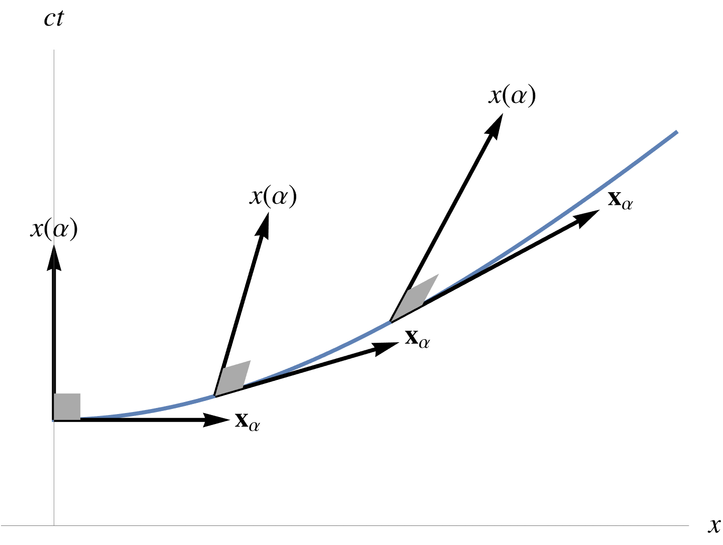
Let \( x = e^{\vcap \alpha/2} \gamma_0 e^{-\vcap \alpha/2} \) represent the spacetime curve of all the boosts of \( \gamma_0 \) along a specific velocity direction vector, where \( \vcap = (v \wedge \gamma_0)/\Norm{v \wedge \gamma_0} \) is a unit spatial bivector for any constant vector \( v \). Compute the line integral
\begin{equation}\label{eqn:fundamentalTheoremOfGC:240}
\int x\, d^1 \Bx.
\end{equation}
Answer
Observe that \( \vcap \) and \( \gamma_0 \) anticommute, so we may write our boost as a one sided exponential
\begin{equation}\label{eqn:fundamentalTheoremOfGC:260}
x(\alpha) = \gamma_0 e^{-\vcap \alpha} = e^{\vcap \alpha} \gamma_0 = \lr{ \cosh\alpha + \vcap \sinh\alpha } \gamma_0.
\end{equation}
The tangent vector is just
\begin{equation}\label{eqn:fundamentalTheoremOfGC:280}
\Bx_\alpha = \PD{\alpha}{x} = e^{\vcap\alpha} \vcap \gamma_0.
\end{equation}
Let’s get a bit of intuition about the nature of this vector. It’s square is
\begin{equation}\label{eqn:fundamentalTheoremOfGC:300}
\begin{aligned}
\Bx_\alpha^2
&=
e^{\vcap\alpha} \vcap \gamma_0
e^{\vcap\alpha} \vcap \gamma_0 \\
&=
-e^{\vcap\alpha} \vcap e^{-\vcap\alpha} \vcap (\gamma_0)^2 \\
&=
-1,
\end{aligned}
\end{equation}
so we see that the tangent vector is a spacelike unit vector. As the vector representing points on the curve is necessarily timelike (due to Lorentz invariance), these two must be orthogonal at all points. Let’s confirm this algebraically
\begin{equation}\label{eqn:fundamentalTheoremOfGC:320}
\begin{aligned}
x \cdot \Bx_\alpha
&=
\gpgradezero{ e^{\vcap \alpha} \gamma_0 e^{\vcap \alpha} \vcap \gamma_0 } \\
&=
\gpgradezero{ e^{-\vcap \alpha} e^{\vcap \alpha} \vcap (\gamma_0)^2 } \\
&=
\gpgradezero{ \vcap } \\
&= 0.
\end{aligned}
\end{equation}
Here we used \( e^{\vcap \alpha} \gamma_0 = \gamma_0 e^{-\vcap \alpha} \), and \( \gpgradezero{A B} = \gpgradezero{B A} \). Geometrically, we have the curious fact that the direction vectors to points on the curve are perpendicular (with respect to our relativistic dot product) to the tangent vectors on the curve, as illustrated in fig. 1.
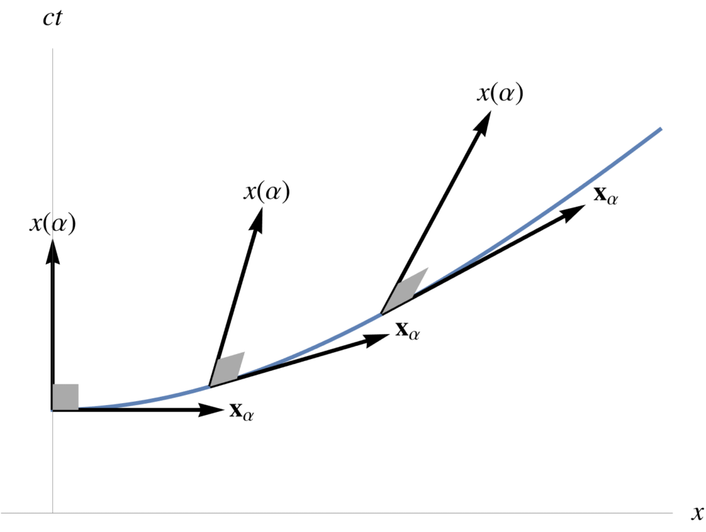
fig. 1. Tangent perpendicularity in mixed metric.
Perfect differentials.
Having seen a couple examples of multivector line integrals, let’s now move on to figure out the structure of a line integral that has a “perfect” differential integrand. We can take a hint from the \(\mathbb{R}^3\) vector result that we already know, namely
\begin{equation}\label{eqn:fundamentalTheoremOfGC:120}
\int_A^B d\Bl \cdot \spacegrad f = f(B) – f(A).
\end{equation}
It seems reasonable to guess that the relativistic generalization of this is
\begin{equation}\label{eqn:fundamentalTheoremOfGC:140}
\int_A^B dx \cdot \grad f = f(B) – f(A).
\end{equation}
Let’s check that, by expanding in coordinates
\begin{equation}\label{eqn:fundamentalTheoremOfGC:160}
\begin{aligned}
\int_A^B dx \cdot \grad f
&=
\int_A^B d\tau \frac{dx^\mu}{d\tau} \partial_\mu f \\
&=
\int_A^B d\tau \frac{dx^\mu}{d\tau} \PD{x^\mu}{f} \\
&=
\int_A^B d\tau \frac{df}{d\tau} \\
&=
f(B) – f(A).
\end{aligned}
\end{equation}
If we drop the dot product, will we have such a nice result? Let’s see:
\begin{equation}\label{eqn:fundamentalTheoremOfGC:180}
\begin{aligned}
\int_A^B dx \grad f
&=
\int_A^B d\tau \frac{dx^\mu}{d\tau} \gamma_\mu \gamma^\nu \partial_\nu f \\
&=
\int_A^B d\tau \frac{dx^\mu}{d\tau} \PD{x^\mu}{f}
+
\int_A^B
d\tau
\sum_{\mu \ne \nu} \gamma_\mu \gamma^\nu
\frac{dx^\mu}{d\tau} \PD{x^\nu}{f}.
\end{aligned}
\end{equation}
This scalar component of this integrand is a perfect differential, but the bivector part of the integrand is a complete mess, that we have no hope of generally integrating. It happens that if we consider one of the simplest parameterization examples, we can get a strong hint of how to generalize the differential operator to one that ends up providing a perfect differential. In particular, let’s integrate over a linear constant path, such as \( x(\tau) = \tau \gamma_0 \). For this path, we have
\begin{equation}\label{eqn:fundamentalTheoremOfGC:200a}
\begin{aligned}
\int_A^B dx \grad f
&=
\int_A^B \gamma_0 d\tau \lr{
\gamma^0 \partial_0 +
\gamma^1 \partial_1 +
\gamma^2 \partial_2 +
\gamma^3 \partial_3 } f \\
&=
\int_A^B d\tau \lr{
\PD{\tau}{f} +
\gamma_0 \gamma^1 \PD{x^1}{f} +
\gamma_0 \gamma^2 \PD{x^2}{f} +
\gamma_0 \gamma^3 \PD{x^3}{f}
}.
\end{aligned}
\end{equation}
Just because the path does not have any \( x^1, x^2, x^3 \) component dependencies does not mean that these last three partials are neccessarily zero. For example \( f = f(x(\tau)) = \lr{ x^0 }^2 \gamma_0 + x^1 \gamma_1 \) will have a non-zero contribution from the \( \partial_1 \) operator. In that particular case, we can easily integrate \( f \), but we have to know the specifics of the function to do the integral. However, if we had a differential operator that did not include any component off the integration path, we would ahve a perfect differential. That is, if we were to replace the gradient with the projection of the gradient onto the tangent space, we would have a perfect differential. We see that the function of the dot product in \ref{eqn:fundamentalTheoremOfGC:140} has the same effect, as it rejects any component of the gradient that does not lie on the tangent space.
Definition 1.2: Vector derivative.
Given a spacetime manifold parameterized by \( x = x(u^0, \cdots u^{N-1}) \), with tangent vectors \( \Bx_\mu = \PDi{u^\mu}{x} \), and reciprocal vectors \( \Bx^\mu \in \textrm{Span}\setlr{\Bx_\nu} \), such that \( \Bx^\mu \cdot \Bx_\nu = {\delta^\mu}_\nu \), the vector derivative is defined as
\begin{equation}\label{eqn:fundamentalTheoremOfGC:240a}
\partial = \sum_{\mu = 0}^{N-1} \Bx^\mu \PD{u^\mu}{}.
\end{equation}
Observe that if this is a full parameterization of the space (\(N = 4\)), then the vector derivative is identical to the gradient. The vector derivative is the projection of the gradient onto the tangent space at the point of evaluation.Furthermore, we designate \( \lrpartial \) as the vector derivative allowed to act bidirectionally, as follows
\begin{equation}\label{eqn:fundamentalTheoremOfGC:260a}
R \lrpartial S
=
R \Bx^\mu \PD{u^\mu}{S}
+
\PD{u^\mu}{R} \Bx^\mu S,
\end{equation}
where \( R, S \) are multivectors, and summation convention is implied. In this bidirectional action,
the vector factors of the vector derivative must stay in place (as they do not neccessarily commute with \( R,S\)), but the derivative operators apply in a chain rule like fashion to both functions.
Noting that \( \Bx_u \cdot \grad = \Bx_u \cdot \partial \), we may rewrite the scalar line integral identity \ref{eqn:fundamentalTheoremOfGC:140} as
\begin{equation}\label{eqn:fundamentalTheoremOfGC:220}
\int_A^B dx \cdot \partial f = f(B) – f(A).
\end{equation}
However, as our example hinted at, the fundamental theorem for line integrals has a multivector generalization that does not rely on a dot product to do the tangent space filtering, and is more powerful. That generalization has the following form.
Theorem 1.1: Fundamental theorem for line integrals.
Given multivector functions \( F, G \), and a single parameter curve \( x(u) \) with line element \( d^1 \Bx = \Bx_u du \), then
\begin{equation}\label{eqn:fundamentalTheoremOfGC:280a}
\int_A^B F d^1\Bx \lrpartial G = F(B) G(B) – F(A) G(A).
\end{equation}
Start proof:
Writing out the integrand explicitly, we find
\begin{equation}\label{eqn:fundamentalTheoremOfGC:340}
\int_A^B F d^1\Bx \lrpartial G
=
\int_A^B \lr{
\PD{\alpha}{F} d\alpha\, \Bx_\alpha \Bx^\alpha G
+
F d\alpha\, \Bx_\alpha \Bx^\alpha \PD{\alpha}{G }
}
\end{equation}
However for a single parameter curve, we have \( \Bx^\alpha = 1/\Bx_\alpha \), so we are left with
\begin{equation}\label{eqn:fundamentalTheoremOfGC:360}
\begin{aligned}
\int_A^B F d^1\Bx \lrpartial G
&=
\int_A^B d\alpha\, \PD{\alpha}{(F G)} \\
&=
\evalbar{F G}{B}
–
\evalbar{F G}{A}.
\end{aligned}
\end{equation}
End proof.
More to come.
In the next installment we will explore surface integrals in spacetime, and the generalization of the fundamental theorem to multivector space time integrals.
References
[1] Peeter Joot. Geometric Algebra for Electrical Engineers. Kindle Direct Publishing, 2019.
[2] A. Macdonald. Vector and Geometric Calculus. CreateSpace Independent Publishing Platform, 2012.
As your T.A., I have to punish you …
December 19, 2020 C/C++ development and debugging. grading comments, horrible code, macros, token pasting
Back in university, I had to implement a reverse polish notation calculator in a software engineering class. Overall the assignment was pretty stupid, and I entertained myself by generating writing a very compact implementation. It worked perfectly, but I got a 25/40 (62.5%) grade on it. That mark was well deserved, although I did not think so at the time.
The grading remarks were actually some of best feedback that I ever received, and also really funny to boot. I don’t know the name of this old now-nameless TA anymore, but I took his advice to heart, and kept his grading remarks on my wall in my IBM office for years. That served as an excellent reminder not to write over complicated code.
Today, I found those remarks again, and am posting them for posterity. Enjoy!
Transcription for easy reading
Reflection.
The only part of this feedback that I would refute was the comment about the string class. That was a actually a pretty good string implementation. I didn’t write it because I was a viscous mouse hunter, but because I hit a porting issue with pre-std:: C. In particular, we had two sets of Solaris machines available to us, and I was using one that had a compiler that included a nice C++ string class. So, naturally I used it. For submission, our code had to compile an run on a different Solaris machine, and lo and behold, the string class that all my code was based on was not available.
What I should have done (20/20 hindsight), was throw out my horrendous code, and start over from scratch. However, I took the more fun approach, and wrote my own string class so that my machine would compile on either machine.
Amusingly, when I worked on IBM LUW, there was a part of the query optimizer code seemed to have learned all it’s tricks from the ugly macros and token pasting that I did in this assignment. It was truly gross, but there was 10000x more of it than my assignment. Having been thoroughly punished for my atrocities, I easily recognized this code for the evil it was. The only way that you could debug that optimizer code, was by running it through the preprocessor, cut and pasting the results, and filtering that cut and paste through something like cindent (these days you would probably use clang-format.) That code was brutal, and I always wished that it’s authors had had the good luck of having a TA like mine. That code is probably still part of LUW terrorizing developers. Apparently the justification for it was that it was originally written by an IBM researcher using templates, but templates couldn’t be used in DB2 code because we didn’t have compiler on all platforms that supported them at the time.
I have used token pasting macros very judiciously and sparingly in the 26 years since I originally used them in this assignment, and I do think that there are a few good uses for that sort of generative code. However, if you do have to write that sort of code, I think it’s better to write perl (or some other language) code that generates understandable code that can be debugged, instead of relying on token pasting.
Share this:
Share on X (Opens in new window)
X
Share on Facebook (Opens in new window)
Facebook
Share on Telegram (Opens in new window)
Telegram
Share on Reddit (Opens in new window)
Reddit
Share on LinkedIn (Opens in new window)
LinkedIn
Email a link to a friend (Opens in new window)
Email
Share on WhatsApp (Opens in new window)
WhatsApp
Like this: