Maxwell equation boundary conditions

September 6, 2016 math and physics play , , , , , , , , , , , , , ,

[Click here for a PDF of this post with nicer formatting]

Motivation

boundaryConditionsTwoSurfacesFig1

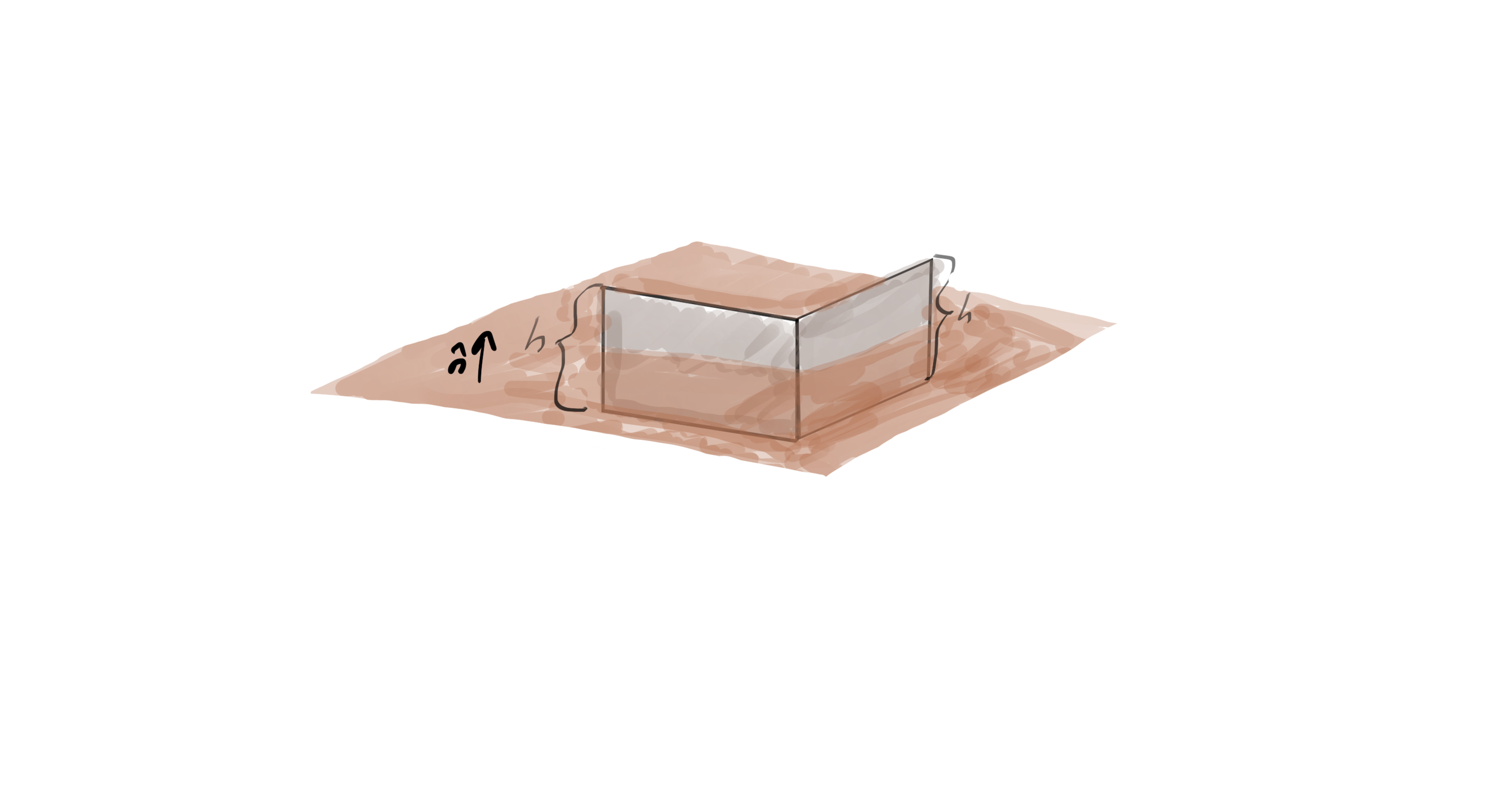
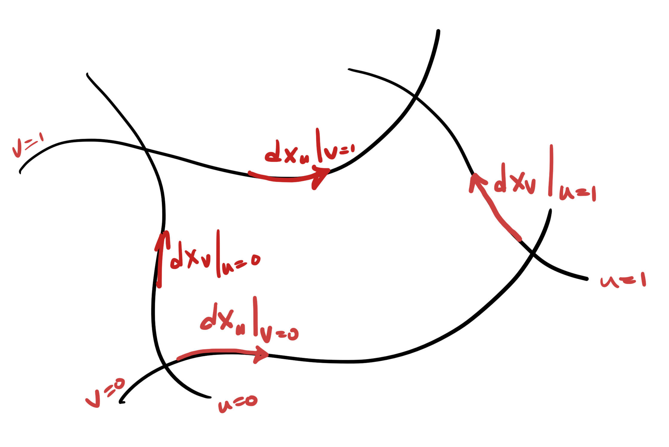
fig 1. Two surfaces normal to the interface.

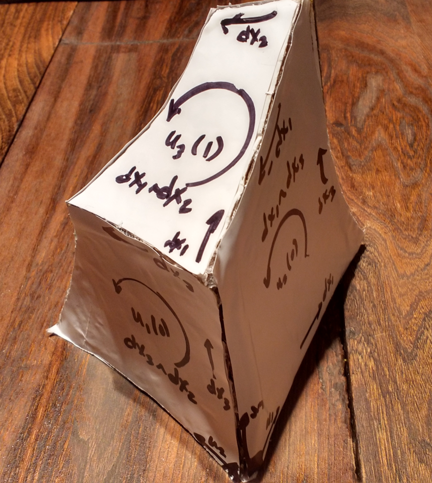
Most electrodynamics textbooks either start with or contain a treatment of boundary value conditions. These typically involve evaluating Maxwell’s equations over areas or volumes of decreasing height, such as those illustrated in fig. 1, and fig. 2. These represent surfaces and volumes where the height is allowed to decrease to infinitesimal levels, and are traditionally used to find the boundary value constraints of the normal and tangential components of the electric and magnetic fields.

boundaryConditionsPillBoxFig2

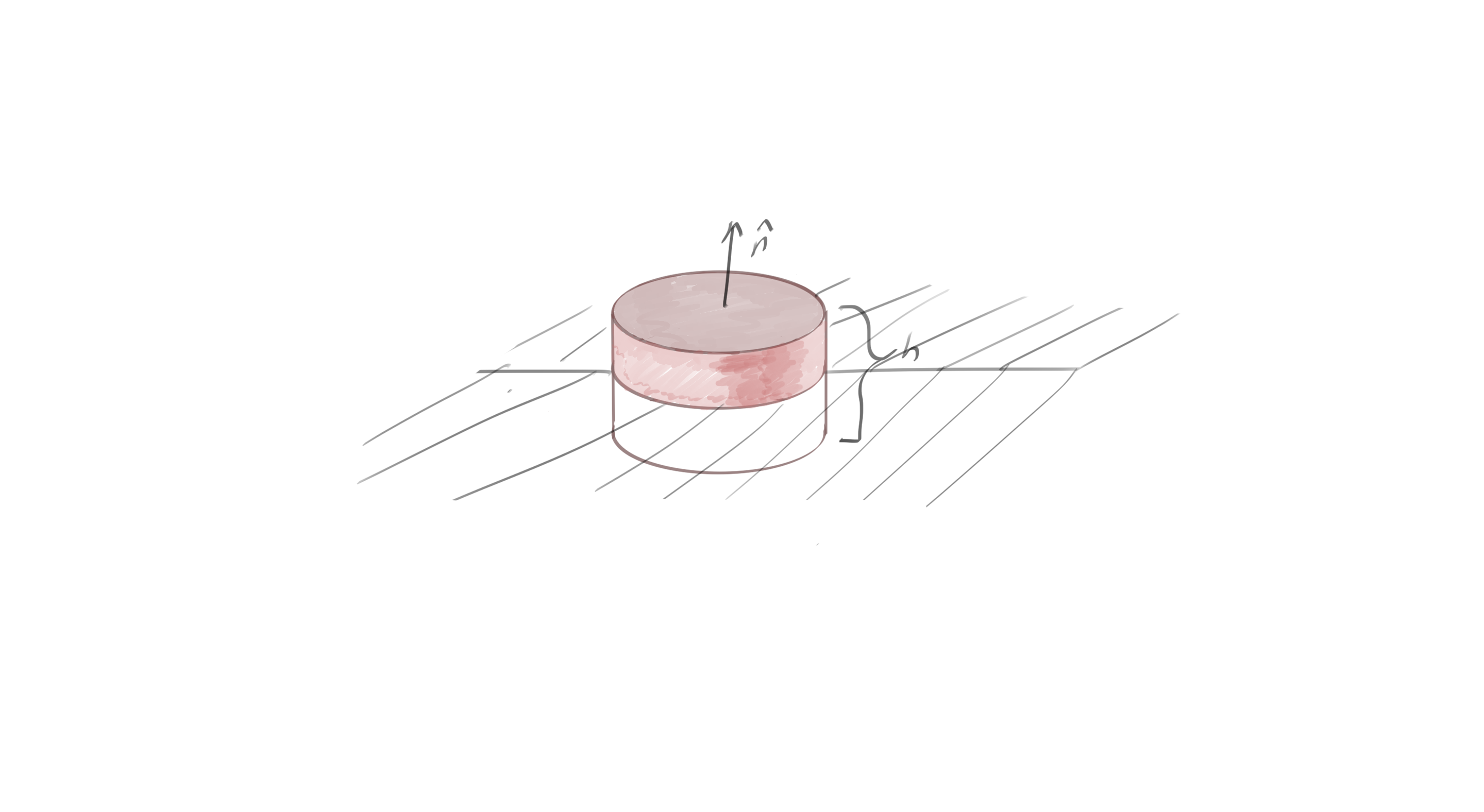
fig 2. A pillbox volume encompassing the interface.

More advanced topics, such as evaluation of the Fresnel reflection and transmission equations, also rely on similar consideration of boundary value constraints. I’ve wondered for a long time how the Fresnel equations could be attacked by looking at the boundary conditions for the combined field \( F = \BE + I c \BB \), instead of the considering them separately.

A unified approach.

The Geometric Algebra (and relativistic tensor) formulations of Maxwell’s equations put the electric and magnetic fields on equal footings. It is in fact possible to specify the boundary value constraints on the fields without first separating Maxwell’s equations into their traditional forms. The starting point in Geometric Algebra is Maxwell’s equation, premultiplied by a stationary observer’s timelike basis vector

\begin{equation}\label{eqn:maxwellBoundaryConditions:20}
\gamma_0 \grad F = \inv{\epsilon_0 c} \gamma_0 J,
\end{equation}

or

\begin{equation}\label{eqn:maxwellBoundaryConditions:40}
\lr{ \partial_0 + \spacegrad} F = \frac{\rho}{\epsilon_0} – \frac{\BJ}{\epsilon_0}.
\end{equation}

The electrodynamic field \(F = \BE + I c \BB\) is a multivector in this spatial domain (whereas it is a bivector in the spacetime algebra domain), and has vector and bivector components. The product of the spatial gradient and the field can still be split into dot and curl components \(\spacegrad M = \spacegrad \cdot M + \spacegrad \wedge M \). If \(M = \sum M_i \), where \(M_i\) is an grade \(i\) blade, then we give this the Hestenes’ [1] definitions

\begin{equation}\label{eqn:maxwellBoundaryConditions:60}
\begin{aligned}
\spacegrad \cdot M &= \sum_i \gpgrade{\spacegrad M_i}{i-1} \\
\spacegrad \wedge M &= \sum_i \gpgrade{\spacegrad M_i}{i+1}.
\end{aligned}
\end{equation}

With that said, Maxwell’s equation can be rearranged into a pair of multivector equations

\begin{equation}\label{eqn:maxwellBoundaryConditions:80}
\begin{aligned}
\spacegrad \cdot F &= \gpgrade{-\partial_0 F + \frac{\rho}{\epsilon_0} – \frac{\BJ}{\epsilon_0 c}}{0,1} \\
\spacegrad \wedge F &= \gpgrade{-\partial_0 F + \frac{\rho}{\epsilon_0} – \frac{\BJ}{\epsilon_0 c}}{2,3},
\end{aligned}
\end{equation}

The latter equation can be integrated with Stokes theorem, but we need to apply a duality transformation to the latter in order to apply Stokes to it

\begin{equation}\label{eqn:maxwellBoundaryConditions:120}
\begin{aligned}
\spacegrad \cdot F
&=
-I^2 \spacegrad \cdot F \\
&=
-I^2 \gpgrade{\spacegrad F}{0,1} \\
&=
-I \gpgrade{I \spacegrad F}{2,3} \\
&=
-I \spacegrad \wedge (IF),
\end{aligned}
\end{equation}

so

\begin{equation}\label{eqn:maxwellBoundaryConditions:100}
\begin{aligned}
\spacegrad \wedge (I F) &= I \lr{ -\inv{c} \partial_t \BE + \frac{\rho}{\epsilon_0} – \frac{\BJ}{\epsilon_0 c} } \\
\spacegrad \wedge F &= -I \partial_t \BB.
\end{aligned}
\end{equation}

Integrating each of these over the pillbox volume gives

\begin{equation}\label{eqn:maxwellBoundaryConditions:140}
\begin{aligned}
\oint_{\partial V} d^2 \Bx \cdot (I F)
&=
\int_{V} d^3 \Bx \cdot \lr{ I \lr{ -\inv{c} \partial_t \BE + \frac{\rho}{\epsilon_0} – \frac{\BJ}{\epsilon_0 c} } } \\
\oint_{\partial V} d^2 \Bx \cdot F
&=
– \partial_t \int_{V} d^3 \Bx \cdot \lr{ I \BB }.
\end{aligned}
\end{equation}

In the absence of charges and currents on the surface, and if the height of the volume is reduced to zero, the volume integrals vanish, and only the upper surfaces of the pillbox contribute to the surface integrals.

\begin{equation}\label{eqn:maxwellBoundaryConditions:200}
\begin{aligned}
\oint_{\partial V} d^2 \Bx \cdot (I F) &= 0 \\
\oint_{\partial V} d^2 \Bx \cdot F &= 0.
\end{aligned}
\end{equation}

With a multivector \(F\) in the mix, the geometric meaning of these integrals is not terribly clear. They do describe the boundary conditions, but to see exactly what those are, we can now resort to the split of \(F\) into its electric and magnetic fields. Let’s look at the non-dual integral to start with

\begin{equation}\label{eqn:maxwellBoundaryConditions:160}
\begin{aligned}
\oint_{\partial V} d^2 \Bx \cdot F
&=
\oint_{\partial V} d^2 \Bx \cdot \lr{ \BE + I c \BB } \\
&=
\oint_{\partial V} d^2 \Bx \cdot \BE + I c d^2 \Bx \wedge \BB \\
&=
0.
\end{aligned}
\end{equation}

No component of \(\BE\) that is normal to the surface contributes to \(d^2 \Bx \cdot \BE \), whereas only components of \(\BB\) that are normal contribute to \(d^2 \Bx \wedge \BB \). That means that we must have tangential components of \(\BE\) and the normal components of \(\BB\) matching on the surfaces

\begin{equation}\label{eqn:maxwellBoundaryConditions:180}
\begin{aligned}
\lr{\BE_2 \wedge \ncap} \ncap – \lr{\BE_1 \wedge (-\ncap)} (-\ncap) &= 0 \\
\lr{\BB_2 \cdot \ncap} \ncap – \lr{\BB_1 \cdot (-\ncap)} (-\ncap) &= 0 .
\end{aligned}
\end{equation}

Similarly, for the dot product of the dual field, this is

\begin{equation}\label{eqn:maxwellBoundaryConditions:220}
\begin{aligned}
\oint_{\partial V} d^2 \Bx \cdot (I F)
&=
\oint_{\partial V} d^2 \Bx \cdot (I \BE – c \BB) \\
&=
\oint_{\partial V} I d^2 \Bx \wedge \BE – c d^2 \Bx \cdot \BB.
\end{aligned}
\end{equation}

For this integral, only the normal components of \(\BE\) contribute, and only the tangential components of \(\BB\) contribute. This means that

\begin{equation}\label{eqn:maxwellBoundaryConditions:240}
\begin{aligned}
\lr{\BE_2 \cdot \ncap} \ncap – \lr{\BE_1 \cdot (-\ncap)} (-\ncap) &= 0 \\
\lr{\BB_2 \wedge \ncap} \ncap – \lr{\BB_1 \wedge (-\ncap)} (-\ncap) &= 0.
\end{aligned}
\end{equation}

This is why we end up with a seemingly strange mix of tangential and normal components of the electric and magnetic fields. These constraints can be summarized as

\begin{equation}\label{eqn:maxwellBoundaryConditions:260}
\begin{aligned}
( \BE_2 – \BE_1 ) \cdot \ncap &= 0 \\
( \BE_2 – \BE_1 ) \wedge \ncap &= 0 \\
( \BB_2 – \BB_1 ) \cdot \ncap &= 0 \\
( \BB_2 – \BB_1 ) \wedge \ncap &= 0
\end{aligned}
\end{equation}

These relationships are usually expressed in terms of all of \(\BE, \BD, \BB\) and \(\BH \). Because I’d started with Maxwell’s equations for free space, I don’t have the \( \epsilon \) and \( \mu \) factors that produce those more general relationships. Those more general boundary value relationships are usually the starting point for the Fresnel interface analysis. It is also possible to further generalize these relationships to include charges and currents on the surface.

References

[1] D. Hestenes. New Foundations for Classical Mechanics. Kluwer Academic Publishers, 1999.

Stokes integrals for Maxwell’s equations in Geometric Algebra

September 4, 2016 math and physics play , , , , , , , , , ,

[Click here for a PDF of this post with nicer formatting]

Recall that the relativistic form of Maxwell’s equation in Geometric Algebra is

\begin{equation}\label{eqn:maxwellStokes:20}
\grad F = \inv{c \epsilon_0} J.
\end{equation}

where \( \grad = \gamma^\mu \partial_\mu \) is the spacetime gradient, and \( J = (c\rho, \BJ) = J^\mu \gamma_\mu \) is the four (vector) current density. The pseudoscalar for the space is denoted \( I = \gamma_0 \gamma_1 \gamma_2 \gamma_3 \), where the basis elements satisfy \( \gamma_0^2 = 1 = -\gamma_k^2 \), and a dual basis satisfies \( \gamma_\mu \cdot \gamma^\nu = \delta_\mu^\nu \). The electromagnetic field \( F \) is a composite multivector \( F = \BE + I c \BB \). This is actually a bivector because spatial vectors have a bivector representation in the space time algebra of the form \( \BE = E^k \gamma_k \gamma_0 \).

Previously, I wrote out the Stokes integrals for Maxwell’s equation in GA form using some three parameter spacetime manifold volumes. This time I’m going to use two and three parameter spatial volumes, again with the Geometric Algebra form of Stokes theorem.

Multiplication by a timelike unit vector transforms Maxwell’s equation from their relativistic form. When that vector is the standard basis timelike unit vector \( \gamma_0 \), we obtain Maxwell’s equations from the point of view of a stationary observer

\begin{equation}\label{eqn:stokesMaxwellSpaceTimeSplit:40}
\lr{\partial_0 + \spacegrad} \lr{ \BE + c I \BB } = \inv{\epsilon_0 c} \lr{ c \rho – \BJ },
\end{equation}

Extracting the scalar, vector, bivector, and trivector grades respectively, we have
\begin{equation}\label{eqn:stokesMaxwellSpaceTimeSplit:60}
\begin{aligned}
\spacegrad \cdot \BE &= \frac{\rho}{\epsilon_0} \\
c I \spacegrad \wedge \BB &= -\partial_0 \BE – \inv{\epsilon_0 c} \BJ \\
\spacegrad \wedge \BE &= – I c \partial_0 \BB \\
c I \spacegrad \cdot \BB &= 0.
\end{aligned}
\end{equation}

Each of these can be written as a curl equation

\begin{equation}\label{eqn:stokesMaxwellSpaceTimeSplit:80}
\boxed{
\begin{aligned}
\spacegrad \wedge (I \BE) &= I \frac{\rho}{\epsilon_0} \\
\inv{\mu_0} \spacegrad \wedge \BB &= \epsilon_0 I \partial_t \BE + I \BJ \\
\spacegrad \wedge \BE &= -I \partial_t \BB \\
\spacegrad \wedge (I \BB) &= 0,
\end{aligned}
}
\end{equation}

a form that allows for direct application of Stokes integrals. The first and last of these require a three parameter volume element, whereas the two bivector grade equations can be integrated using either two or three parameter volume elements. Suppose that we have can parameterize the space with parameters \( u, v, w \), for which the gradient has the representation

\begin{equation}\label{eqn:stokesMaxwellSpaceTimeSplit:100}
\spacegrad = \Bx^u \partial_u + \Bx^v \partial_v + \Bx^w \partial_w,
\end{equation}

but we integrate over a two parameter subset of this space spanned by \( \Bx(u,v) \), with area element

\begin{equation}\label{eqn:stokesMaxwellSpaceTimeSplit:120}
\begin{aligned}
d^2 \Bx
&= d\Bx_u \wedge d\Bx_v \\
&=
\PD{u}{\Bx}
\wedge
\PD{v}{\Bx}
\,du dv \\
&=
\Bx_u
\wedge
\Bx_v
\,du dv,
\end{aligned}
\end{equation}

as illustrated in fig. 1.


twoParameterAreaElementFig1

fig. 1. Two parameter manifold.

Our curvilinear coordinates \( \Bx_u, \Bx_v, \Bx_w \) are dual to the reciprocal basis \( \Bx^u, \Bx^v, \Bx^w \), but we won’t actually have to calculate that reciprocal basis. Instead we need only know that it can be calculated and is defined by the relations \( \Bx_a \cdot \Bx^b = \delta_a^b \). Knowing that we can reduce (say),

\begin{equation}\label{eqn:stokesMaxwellSpaceTimeSplit:140}
\begin{aligned}
d^2 \Bx \cdot ( \spacegrad \wedge \BE )
&=
d^2 \Bx \cdot ( \Bx^a \partial_a \wedge \BE ) \\
&=
(\Bx_u \wedge \Bx_v) \cdot ( \Bx^a \wedge \partial_a \BE ) \,du dv \\
&=
(((\Bx_u \wedge \Bx_v) \cdot \Bx^a) \cdot \partial_a \BE \,du dv \\
&=
d\Bx_u \cdot \partial_v \BE \,dv
-d\Bx_v \cdot \partial_u \BE \,du,
\end{aligned}
\end{equation}

Because each of the differentials, for example \( d\Bx_u = (\PDi{u}{\Bx}) du \), is calculated with the other (i.e.\( v \)) held constant, this is directly integrable, leaving

\begin{equation}\label{eqn:stokesMaxwellSpaceTimeSplit:160}
\begin{aligned}
\int d^2 \Bx \cdot ( \spacegrad \wedge \BE )
&=
\int \evalrange{\lr{d\Bx_u \cdot \BE}}{v=0}{v=1}
-\int \evalrange{\lr{d\Bx_v \cdot \BE}}{u=0}{u=1} \\
&=
\oint d\Bx \cdot \BE.
\end{aligned}
\end{equation}

That direct integration of one of the parameters, while the others are held constant, is the basic idea behind Stokes theorem.

The pseudoscalar grade Maxwell’s equations from \ref{eqn:stokesMaxwellSpaceTimeSplit:80} require a three parameter volume element to apply Stokes theorem to. Again, allowing for curvilinear coordinates such a differential expands as

\begin{equation}\label{eqn:stokesMaxwellSpaceTimeSplit:180}
\begin{aligned}
d^3 \Bx \cdot (\spacegrad \wedge (I\BB))
&=
(( \Bx_u \wedge \Bx_v \wedge \Bx_w ) \cdot \Bx^a ) \cdot \partial_a (I\BB) \,du dv dw \\
&=
(d\Bx_u \wedge d\Bx_v) \cdot \partial_w (I\BB) dw
+(d\Bx_v \wedge d\Bx_w) \cdot \partial_u (I\BB) du
+(d\Bx_w \wedge d\Bx_u) \cdot \partial_v (I\BB) dv.
\end{aligned}
\end{equation}

Like the two parameter volume, this is directly integrable

\begin{equation}\label{eqn:stokesMaxwellSpaceTimeSplit:200}
\int
d^3 \Bx \cdot (\spacegrad \wedge (I\BB))
=
\int \evalbar{(d\Bx_u \wedge d\Bx_v) \cdot (I\BB) }{\Delta w}
+\int \evalbar{(d\Bx_v \wedge d\Bx_w) \cdot (I\BB)}{\Delta u}
+\int \evalbar{(d\Bx_w \wedge d\Bx_u) \cdot (I\BB)}{\Delta v}.
\end{equation}

After some thought (or a craft project such as that of fig. 2) is can be observed that this is conceptually an oriented surface integral

threeParameterSurfaceFig2

fig. 2. Oriented three parameter surface.

Noting that

\begin{equation}\label{eqn:stokesMaxwellSpaceTimeSplit:221}
\begin{aligned}
d^2 \Bx \cdot (I\Bf)
&= \gpgradezero{ d^2 \Bx I B } \\
&= I (d^2\Bx \wedge \Bf)
\end{aligned}
\end{equation}

we can now write down the results of application of Stokes theorem to each of Maxwell’s equations in their curl forms

\begin{equation}\label{eqn:stokesMaxwellSpaceTimeSplit:220}
\boxed{
\begin{aligned}
\oint d\Bx \cdot \BE &= -I \partial_t \int d^2 \Bx \wedge \BB \\
\inv{\mu_0} \oint d\Bx \cdot \BB &= \epsilon_0 I \partial_t \int d^2 \Bx \wedge \BE + I \int d^2 \Bx \wedge \BJ \\
\oint d^2 \Bx \wedge \BE &= \inv{\epsilon_0} \int (d^3 \Bx \cdot I) \rho \\
\oint d^2 \Bx \wedge \BB &= 0.
\end{aligned}
}
\end{equation}

In the three parameter surface integrals the specific meaning to apply to \( d^2 \Bx \wedge \Bf \) is
\begin{equation}\label{eqn:stokesMaxwellSpaceTimeSplit:240}
\oint d^2 \Bx \wedge \Bf
=
\int \evalbar{\lr{d\Bx_u \wedge d\Bx_v \wedge \Bf}}{\Delta w}
+\int \evalbar{\lr{d\Bx_v \wedge d\Bx_w \wedge \Bf}}{\Delta u}
+\int \evalbar{\lr{d\Bx_w \wedge d\Bx_u \wedge \Bf}}{\Delta v}.
\end{equation}

Note that in each case only the component of the vector \( \Bf \) that is projected onto the normal to the area element contributes.

Application of Stokes Theorem to the Maxwell equation

September 3, 2016 math and physics play , , , , , , , , , , , ,

[Click here for a PDF of this post with nicer formatting]

The relativistic form of Maxwell’s equation in Geometric Algebra is

\begin{equation}\label{eqn:maxwellStokes:20}
\grad F = \inv{c \epsilon_0} J,
\end{equation}

where \( \grad = \gamma^\mu \partial_\mu \) is the spacetime gradient, and \( J = (c\rho, \BJ) = J^\mu \gamma_\mu \) is the four (vector) current density. The pseudoscalar for the space is denoted \( I = \gamma_0 \gamma_1 \gamma_2 \gamma_3 \), where the basis elements satisfy \( \gamma_0^2 = 1 = -\gamma_k^2 \), and a dual basis satisfies \( \gamma_\mu \cdot \gamma^\nu = \delta_\mu^\nu \). The electromagnetic field \( F \) is a composite multivector \( F = \BE + I c \BB \). This is actually a bivector because spatial vectors have a bivector representation in the space time algebra of the form \( \BE = E^k \gamma_k \gamma_0 \).

A dual representation, with \( F = I G \) is also possible

\begin{equation}\label{eqn:maxwellStokes:60}
\grad G = \frac{I}{c \epsilon_0} J.
\end{equation}

Either form of Maxwell’s equation can be split into grade one and three components. The standard (non-dual) form is

\begin{equation}\label{eqn:maxwellStokes:40}
\begin{aligned}
\grad \cdot F &= \inv{c \epsilon_0} J \\
\grad \wedge F &= 0,
\end{aligned}
\end{equation}

and the dual form is

\begin{equation}\label{eqn:maxwellStokes:41}
\begin{aligned}
\grad \cdot G &= 0 \\
\grad \wedge G &= \frac{I}{c \epsilon_0} J.
\end{aligned}
\end{equation}

In both cases a potential representation \( F = \grad \wedge A \), where \( A \) is a four vector potential can be used to kill off the non-current equation. Such a potential representation reduces Maxwell’s equation to

\begin{equation}\label{eqn:maxwellStokes:80}
\grad \cdot F = \inv{c \epsilon_0} J,
\end{equation}

or
\begin{equation}\label{eqn:maxwellStokes:100}
\grad \wedge G = \frac{I}{c \epsilon_0} J.
\end{equation}

In both cases, these reduce to
\begin{equation}\label{eqn:maxwellStokes:120}
\grad^2 A – \grad \lr{ \grad \cdot A } = \inv{c \epsilon_0} J.
\end{equation}

This can clearly be further simplified by using the Lorentz gauge, where \( \grad \cdot A = 0 \). However, the aim for now is to try applying Stokes theorem to Maxwell’s equation. The dual form \ref{eqn:maxwellStokes:100} has the curl structure required for the application of Stokes. Suppose that we evaluate this curl over the three parameter volume element \( d^3 x = i\, dx^0 dx^1 dx^2 \), where \( i = \gamma_0 \gamma_1 \gamma_2 \) is the unit pseudoscalar for the spacetime volume element.

\begin{equation}\label{eqn:maxwellStokes:101}
\begin{aligned}
\int_V d^3 x \cdot \lr{ \grad \wedge G }
&=
\int_V d^3 x \cdot \lr{ \gamma^\mu \wedge \partial_\mu G } \\
&=
\int_V \lr{ d^3 x \cdot \gamma^\mu } \cdot \partial_\mu G \\
&=
\sum_{\mu \ne 3} \int_V \lr{ d^3 x \cdot \gamma^\mu } \cdot \partial_\mu G.
\end{aligned}
\end{equation}

This uses the distibution identity \( A_s \cdot (a \wedge A_r) = (A_s \cdot a) \cdot A_r \) which holds for blades \( A_s, A_r \) provided \( s > r > 0 \). Observe that only the component of the gradient that lies in the tangent space of the three volume manifold contributes to the integral, allowing the gradient to be used in the Stokes integral instead of the vector derivative (see: [1]).
Defining the the surface area element

\begin{equation}\label{eqn:maxwellStokes:140}
\begin{aligned}
d^2 x
&= \sum_{\mu \ne 3} i \cdot \gamma^\mu \inv{dx^\mu} d^3 x \\
&= \gamma_1 \gamma_2 dx dy
+ c \gamma_2 \gamma_0 dt dy
+ c \gamma_0 \gamma_1 dt dx,
\end{aligned}
\end{equation}

Stokes theorem for this volume element is now completely specified

\begin{equation}\label{eqn:maxwellStokes:200}
\int_V d^3 x \cdot \lr{ \grad \wedge G }
=
\int_{\partial V} d^2 \cdot G.
\end{equation}

Application to the dual Maxwell equation gives

\begin{equation}\label{eqn:maxwellStokes:160}
\int_{\partial V} d^2 x \cdot G
= \inv{c \epsilon_0} \int_V d^3 x \cdot (I J).
\end{equation}

After some manipulation, this can be restated in the non-dual form

\begin{equation}\label{eqn:maxwellStokes:180}
\boxed{
\int_{\partial V} \inv{I} d^2 x \wedge F
= \frac{1}{c \epsilon_0 I} \int_V d^3 x \wedge J.
}
\end{equation}

It can be demonstrated that using this with each of the standard basis spacetime 3-volume elements recovers Gauss’s law and the Ampere-Maxwell equation. So, what happened to Faraday’s law and Gauss’s law for magnetism? With application of Stokes to the curl equation from \ref{eqn:maxwellStokes:40}, those equations take the form

\begin{equation}\label{eqn:maxwellStokes:240}
\boxed{
\int_{\partial V} d^2 x \cdot F = 0.
}
\end{equation}

Problem 1:

Demonstrate that the Ampere-Maxwell equation and Gauss’s law can be recovered from the trivector (curl) equation \ref{eqn:maxwellStokes:100}.

Answer

The curl equation is a trivector on each side, so dotting it with each of the four possible trivectors \( \gamma_0 \gamma_1 \gamma_2, \gamma_0 \gamma_2 \gamma_3, \gamma_0 \gamma_1 \gamma_3, \gamma_1 \gamma_2 \gamma_3 \) will give four different scalar equations. For example, dotting with \( \gamma_0 \gamma_1 \gamma_2 \), we have for the curl side

\begin{equation}\label{eqn:maxwellStokes:460}
\begin{aligned}
\lr{ \gamma_0 \gamma_1 \gamma_2 } \cdot \lr{ \gamma^\mu \wedge \partial_\mu G }
&=
\lr{ \lr{ \gamma_0 \gamma_1 \gamma_2 } \cdot \gamma^\mu } \cdot \partial_\mu G \\
&=
(\gamma_0 \gamma_1) \cdot \partial_2 G
+(\gamma_2 \gamma_0) \cdot \partial_1 G
+(\gamma_1 \gamma_2) \cdot \partial_0 G,
\end{aligned}
\end{equation}

and for the current side, we have

\begin{equation}\label{eqn:maxwellStokes:480}
\begin{aligned}
\inv{\epsilon_0 c} \lr{ \gamma_0 \gamma_1 \gamma_2 } \cdot \lr{ I J }
&=
\inv{\epsilon_0 c} \gpgradezero{ \gamma_0 \gamma_1 \gamma_2 (\gamma_0 \gamma_1 \gamma_2 \gamma_3) J } \\
&=
\inv{\epsilon_0 c} \gpgradezero{ -\gamma_3 J } \\
&=
\inv{\epsilon_0 c} \gamma^3 \cdot J \\
&=
\inv{\epsilon_0 c} J^3,
\end{aligned}
\end{equation}

so we have
\begin{equation}\label{eqn:maxwellStokes:500}
(\gamma_0 \gamma_1) \cdot \partial_2 G
+(\gamma_2 \gamma_0) \cdot \partial_1 G
+(\gamma_1 \gamma_2) \cdot \partial_0 G
=
\inv{\epsilon_0 c} J^3.
\end{equation}

Similarily, dotting with \( \gamma_{013}, \gamma_{023}, and \gamma_{123} \) respectively yields
\begin{equation}\label{eqn:maxwellStokes:620}
\begin{aligned}
\gamma_{01} \cdot \partial_3 G + \gamma_{30} \partial_1 G + \gamma_{13} \partial_0 G &= – \inv{\epsilon_0 c} J^2 \\
\gamma_{02} \cdot \partial_3 G + \gamma_{30} \partial_2 G + \gamma_{23} \partial_0 G &= \inv{\epsilon_0 c} J^1 \\
\gamma_{12} \cdot \partial_3 G + \gamma_{31} \partial_2 G + \gamma_{23} \partial_1 G &= -\inv{\epsilon_0} \rho.
\end{aligned}
\end{equation}

Expanding the dual electromagnetic field, first in terms of the spatial vectors, and then in the space time basis, we have
\begin{equation}\label{eqn:maxwellStokes:520}
\begin{aligned}
G
&= -I F \\
&= -I \lr{ \BE + I c \BB } \\
&= -I \BE + c \BB. \\
&= -I \BE + c B^k \gamma_k \gamma_0 \\
&= \inv{2} \epsilon^{r s t} \gamma_r \gamma_s E^t + c B^k \gamma_k \gamma_0.
\end{aligned}
\end{equation}

So, dotting with a spatial vector will pick up a component of \( \BB \), we have
\begin{equation}\label{eqn:maxwellStokes:540}
\begin{aligned}
\lr{ \gamma_m \wedge \gamma_0 } \cdot \partial_\mu G
&=
\lr{ \gamma_m \wedge \gamma_0 } \cdot \partial_\mu \lr{
\inv{2} \epsilon^{r s t} \gamma_r \gamma_s E^t + c B^k \gamma_k \gamma_0
} \\
&=
c \partial_\mu B^k
\gpgradezero{
\gamma_m \gamma_0 \gamma_k \gamma_0
} \\
&=
c \partial_\mu B^k
\gpgradezero{
\gamma_m \gamma_0 \gamma_0 \gamma^k
} \\
&=
c \partial_\mu B^k
\delta_m^k \\
&=
c \partial_\mu B^m.
\end{aligned}
\end{equation}

Written out explicitly the electric field contributions to \( G \) are

\begin{equation}\label{eqn:maxwellStokes:560}
\begin{aligned}
-I \BE
&=
-\gamma_{0123k0} E^k \\
&=
-\gamma_{123k} E^k \\
&=
\left\{
\begin{array}{l l}
\gamma_{12} E^3 & \quad \mbox{\( k = 3 \)} \\
\gamma_{31} E^2 & \quad \mbox{\( k = 2 \)} \\
\gamma_{23} E^1 & \quad \mbox{\( k = 1 \)} \\
\end{array}
\right.,
\end{aligned}
\end{equation}

so
\begin{equation}\label{eqn:maxwellStokes:580}
\begin{aligned}
\gamma_{23} \cdot G &= -E^1 \\
\gamma_{31} \cdot G &= -E^2 \\
\gamma_{12} \cdot G &= -E^3.
\end{aligned}
\end{equation}

We now have the pieces required to expand \ref{eqn:maxwellStokes:500} and \ref{eqn:maxwellStokes:620}, which are respectively

\begin{equation}\label{eqn:maxwellStokes:501}
\begin{aligned}
– c \partial_2 B^1 + c \partial_1 B^2 – \partial_0 E^3 &= \inv{\epsilon_0 c} J^3 \\
– c \partial_3 B^1 + c \partial_1 B^3 + \partial_0 E^2 &= -\inv{\epsilon_0 c} J^2 \\
– c \partial_3 B^2 + c \partial_2 B^3 – \partial_0 E^1 &= \inv{\epsilon_0 c} J^1 \\
– \partial_3 E^3 – \partial_2 E^2 – \partial_1 E^1 &= – \inv{\epsilon_0} \rho
\end{aligned}
\end{equation}

which are the components of the Ampere-Maxwell equation, and Gauss’s law

\begin{equation}\label{eqn:maxwellStokes:600}
\begin{aligned}
\inv{\mu_0} \spacegrad \cross \BB – \epsilon_0 \PD{t}{\BE} &= \BJ \\
\spacegrad \cdot \BE &= \frac{\rho}{\epsilon_0}.
\end{aligned}
\end{equation}

Problem 2:

Prove \ref{eqn:maxwellStokes:180}.

Answer

The proof just requires the expansion of the dot products using scalar selection

\begin{equation}\label{eqn:maxwellStokes:260}
\begin{aligned}
d^2 x \cdot G
&=
\gpgradezero{ d^2 x (-I) F } \\
&=
-\gpgradezero{ I d^2 x F } \\
&=
-I \lr{ d^2 x \wedge F },
\end{aligned}
\end{equation}

and
for the three volume dot product

\begin{equation}\label{eqn:maxwellStokes:280}
\begin{aligned}
d^3 x \cdot (I J)
&=
\gpgradezero{
d^3 x\, I J
} \\
&=
-\gpgradezero{
I d^3 x\, J
} \\
&=
-I \lr{ d^3 x \wedge J }.
\end{aligned}
\end{equation}

Problem 3:

Using each of the four possible spacetime volume elements, write out the components of the Stokes integral
\ref{eqn:maxwellStokes:180}.

Answer

The four possible volume and associated area elements are
\begin{equation}\label{eqn:maxwellStokes:220}
\begin{aligned}
d^3 x = c \gamma_0 \gamma_1 \gamma_2 dt dx dy & \qquad d^2 x = \gamma_1 \gamma_2 dx dy + c \gamma_2 \gamma_0 dy dt + c \gamma_0 \gamma_1 dt dx \\
d^3 x = c \gamma_0 \gamma_1 \gamma_3 dt dx dz & \qquad d^2 x = \gamma_1 \gamma_3 dx dz + c \gamma_3 \gamma_0 dz dt + c \gamma_0 \gamma_1 dt dx \\
d^3 x = c \gamma_0 \gamma_2 \gamma_3 dt dy dz & \qquad d^2 x = \gamma_2 \gamma_3 dy dz + c \gamma_3 \gamma_0 dz dt + c \gamma_0 \gamma_2 dt dy \\
d^3 x = \gamma_1 \gamma_2 \gamma_3 dx dy dz & \qquad d^2 x = \gamma_1 \gamma_2 dx dy + \gamma_2 \gamma_3 dy dz + c \gamma_3 \gamma_1 dz dx \\
\end{aligned}
\end{equation}

Wedging the area element with \( F \) will produce pseudoscalar multiples of the various \( \BE \) and \( \BB \) components, but a recipe for these components is required.

First note that for \( k \ne 0 \), the wedge \( \gamma_k \wedge \gamma_0 \wedge F \) will just select components of \( \BB \). This can be seen first by simplifying

\begin{equation}\label{eqn:maxwellStokes:300}
\begin{aligned}
I \BB
&=
\gamma_{0 1 2 3} B^m \gamma_{m 0} \\
&=
\left\{
\begin{array}{l l}
\gamma_{3 2} B^1 & \quad \mbox{\( m = 1 \)} \\
\gamma_{1 3} B^2 & \quad \mbox{\( m = 2 \)} \\
\gamma_{2 1} B^3 & \quad \mbox{\( m = 3 \)}
\end{array}
\right.,
\end{aligned}
\end{equation}

or

\begin{equation}\label{eqn:maxwellStokes:320}
I \BB = – \epsilon_{a b c} \gamma_{a b} B^c.
\end{equation}

From this it follows that

\begin{equation}\label{eqn:maxwellStokes:340}
\gamma_k \wedge \gamma_0 \wedge F = I c B^k.
\end{equation}

The electric field components are easier to pick out. Those are selected by

\begin{equation}\label{eqn:maxwellStokes:360}
\begin{aligned}
\gamma_m \wedge \gamma_n \wedge F
&= \gamma_m \wedge \gamma_n \wedge \gamma_k \wedge \gamma_0 E^k \\
&= -I E^k \epsilon_{m n k}.
\end{aligned}
\end{equation}

The respective volume element wedge products with \( J \) are

\begin{equation}\label{eqn:maxwellStokes:400}
\begin{aligned}
\inv{I} d^3 x \wedge J = \inv{c \epsilon_0} J^3
\inv{I} d^3 x \wedge J = \inv{c \epsilon_0} J^2
\inv{I} d^3 x \wedge J = \inv{c \epsilon_0} J^1,
\end{aligned}
\end{equation}

and the respective sum of surface area elements wedged with the electromagnetic field are

\begin{equation}\label{eqn:maxwellStokes:380}
\begin{aligned}
\inv{I} d^2 x \wedge F &= – \evalbar{E^3}{c \Delta t} dx dy + c \lr{ \evalbar{B^2}{\Delta x} dy – \evalbar{B^1}{\Delta y} dx } dt \\
\inv{I} d^2 x \wedge F &= \evalbar{E^2}{c \Delta t} dx dz + c \lr{ \evalbar{B^3}{\Delta x} dz – \evalbar{B^1}{\Delta z} dx } dt \\
\inv{I} d^2 x \wedge F &= – \evalbar{E^1}{c \Delta t} dy dz + c \lr{ \evalbar{B^3}{\Delta y} dz – \evalbar{B^2}{\Delta z} dy } dt \\
\inv{I} d^2 x \wedge F &= – \evalbar{E^3}{\Delta z} dy dx – \evalbar{E^2}{\Delta y} dx dz – \evalbar{E^1}{\Delta x} dz dy,
\end{aligned}
\end{equation}

so
\begin{equation}\label{eqn:maxwellStokes:381}
\begin{aligned}
\int_{\partial V} – \evalbar{E^3}{c \Delta t} dx dy + c \lr{ \evalbar{B^2}{\Delta x} dy – \evalbar{B^1}{\Delta y} dx } dt &=
c \int_V dx dy dt \inv{c \epsilon_0} J^3 \\
\int_{\partial V} \evalbar{E^2}{c \Delta t} dx dz + c \lr{ \evalbar{B^3}{\Delta x} dz – \evalbar{B^1}{\Delta z} dx } dt &=
-c \int_V dx dy dt \inv{c \epsilon_0} J^2 \\
\int_{\partial V} – \evalbar{E^1}{c \Delta t} dy dz + c \lr{ \evalbar{B^3}{\Delta y} dz – \evalbar{B^2}{\Delta z} dy } dt &=
c \int_V dx dy dt \inv{c \epsilon_0} J^1 \\
\int_{\partial V} – \evalbar{E^3}{\Delta z} dy dx – \evalbar{E^2}{\Delta y} dx dz – \evalbar{E^1}{\Delta x} dz dy &=
-\int_V dx dy dz \inv{\epsilon_0} \rho.
\end{aligned}
\end{equation}

Observe that if the volume elements are taken to their infinesimal limits, we recover the traditional differential forms of the Ampere-Maxwell and Gauss’s law equations.

References

[1] A. Macdonald. Vector and Geometric Calculus. CreateSpace Independent Publishing Platform, 2012.

brace matching in vim, regardless of how it is formatted?

August 31, 2016 C/C++ development and debugging. ,

DB2 functions were usually formatted with the brace on the leading line like so:

size_t table_count( T * table )
{ 
   size_t count = 0 ;
   ....
} 

For such code, typing [[ in vim anywhere from somewhere in the function text would take you to the beginning of the function. It has always annoyed me that this key sequence didn’t work for functions formatted without the leading { in the first column, such as

size_t table_count( T * table ) { 
    size_t count = 0 ;
    ....
} 

Having my handy [[ command sequence take me to the first line of the file is pretty annoying, enough that I looked up the way to do what I want. A key sequence that does part of this job is:

[{

This takes you to the outermost ending position of the current scope, and you can use % to get to the beginning of that scope. You can repeat this as many times as necessary, until you get the outermost scope.

Is there a better way to go directly to the outermost scope directly, regardless of how the function happens to be formatted?

New home office and network setup

August 30, 2016 Uncategorized

I’ve just bought a nice new desk for my home office:

IMG_20160830_123415866_HDR

When I assembled the new desk, I took the opportunity to refine my home network setup. In this post I’ll walk through that setup.

I’ve got the router in the living room, along with the two NUC6i’s that I use for my lzlabs development work:

nucs and router

I run the NUCs headless, using ssh and command line access for my work. For those times that I need to refresh the install image and need a display, I also have them HDMI connected to the living room TV, and direct connected with short ethernet cables to the router:

nuc wiring

The router is also directly connected to the PS3 (for netflix), and then runs through some ethernet lines that I fished into the basement, before some of the basement finishing work we did just after we moved in. All the lines I have going into the basement terminate in a patch panel:

patch panel

Does a patch panel sound like overkill? Yes, it probably is. However, I’ve got a pile of roughed in ethernet lines to the kids rooms and the rec room that I’ll eventually fish into the electrical-panel/laundry/network room:

wire bundle

I’d like to also eventually fish some ethernet lines into the upstairs space (i.e. for netflix run off a blue-ray player that sits mostly unused in the master bedroom), but that’s a harder fishing job, and I haven’t done it yet. From the front of the patch panel things go off to the router:

patch panel 2

and from there to a switch:

switch and phone

One line comes from the router (through the patch panel), and then all the rest of the ethernet lines from the switch go to final destinations. Four of those lines go back to the patch panel and up to the office space. One is plugged into one of the thunderbolt monitors, so I can use a wired connection while “docked”. One goes up to the office space and is connected to an Odroid (which can run the Lz stack on aarch64 hardware). One line goes back to the living room, for optional wired couch surfing, and the last is connected to a voip phone.

I’ve got a lot of finishing touches to do. I plan to mount the patch panel next to the electrical panel, instead of just placing it on top of the freezer down in the laundry room. I’ve also got lines that are running through the ceiling, but are hanging loose still. The wall panel in my office space is currently hanging loose:

desk cabling

I have a low voltage wiring box purchased, but need to cut the hole for it, so I can screw in this little panel and get it nicely out of the way, and do the plastering and painting to fix up the messy fishing holes I made trying to find a route down into the basement.