contour integral

A Green’s function solution to falling with resistance problem.

January 30, 2025 math and physics play , , , , , , , ,

[Click here for a PDF version of this post]

Motivation.

In a fun twitter/x post, we have a Green’s function solution to a constant acceleration problem with drag. The post is meant to be a joke, as the stated problem is: “A boy drops a ball from a height \( h \). What is the speed of the ball when it reaches the floor (no drag)?”

The joke is that nobody would solve this problem using Green’s functions, and nobody would solve this function using Green’s functions for the more general case, allowing for drag. Instead, you’d just solve this using energy balance, which makes the problem trivial.

That said, there are actually lots of cool ideas in the Green’s function method on the joke side of the solution.

So let’s play along with the joke and solve the general damped problem with Green’s functions. Along the way, we can fill in the missing details, and also explore some supplemental ideas that are worth understanding.

Setup.

The equation of motion is
\begin{equation}\label{eqn:greensDropWithResistance:20}
m \frac{d^2 \Bx}{dt^2} = – \gamma \frac{d \Bx}{dt} – m \Bg,
\end{equation}
where \( \Bg \) is a constant (positively oriented) force. The first detail that needs to be included, is that this isn’t the differential equation for the stated problem, and will become problematic should we attempt to apply Green’s function methods. We have to account for the “boy drops” part of the problem statement, and solve with a different forcing function, namely
\begin{equation}\label{eqn:greensDropWithResistance:40}
m \frac{d^2 \Bx}{dt^2} = – \gamma \frac{d \Bx}{dt} – m \Bg \Theta(t).
\end{equation}
This revised model of the system begins the application of the constant (gravitational) force, at time \( t = 0 \). This is now a system that will yield to Green’s function methods.

Fourier transform solution.

The joke solution has strong hints that Fourier transform methods were part of the story. In particular, it appears that the following definitions of the transform pair were used
\begin{equation}\label{eqn:greensDropWithResistance:60}
\begin{aligned}
\hatU(\omega) = F(u(t)) &= \int_{-\infty}^\infty u(t) e^{-i\omega t} dt \\
u(t) = F^{-1}(\hatU(\omega)) &= \inv{2\pi} \int_{-\infty}^\infty \hatU(\omega) e^{i\omega t} d\omega.
\end{aligned}
\end{equation}
However, if we are using Fourier transforms, why bother with Green’s functions? Instead, we can just solve for the system response using Fourier transforms. When looking for the system response, we usually pose the problem with more generality. For example, instead of the specific theta-weighted constant gravitational forcing function above, we seek to find the solution of
\begin{equation}\label{eqn:greensDropWithResistance:80}
m \frac{d^2 \Bx}{dt^2} + \gamma \frac{d \Bx}{dt} = \BF(t).
\end{equation}
We start by assuming that the Fourier transforms of \( \Bx(t), \BF(t) \) are \( \hat{\BX}(\omega), \hat{\BF}(\omega) \) so
\begin{equation}\label{eqn:greensDropWithResistance:100}
\Bx(t) = \inv{2\pi} \int_{-\infty}^\infty e^{i\omega t} \hat{\BX}(\omega) d\omega.
\end{equation}
Derivatives of this presumed Fourier representation are trivial
\begin{equation}\label{eqn:greensDropWithResistance:120}
\begin{aligned}
\Bx'(t) &= \inv{2\pi} \int_{-\infty}^\infty \lr{ i\omega } e^{i\omega t} \hat{\BX}(\omega) d\omega \\
\Bx”(t) &= \inv{2\pi} \int_{-\infty}^\infty \lr{ i\omega }^2 e^{i\omega t} \hat{\BX}(\omega) d\omega,
\end{aligned}
\end{equation}
so the frequency representation of our system is
\begin{equation}\label{eqn:greensDropWithResistance:140}
\inv{2\pi} \int_{-\infty}^\infty \lr{ m \lr{ i\omega }^2 + \gamma \lr{ i\omega} } e^{i\omega t} \hat{\BX}(\omega) d\omega
=
\inv{2\pi} \int_{-\infty}^\infty e^{i\omega t} \hat{\BF}(\omega) d\omega,
\end{equation}
or
\begin{equation}\label{eqn:greensDropWithResistance:160}
\hat{\BX}(\omega) = \frac{\hat{\BF}(\omega)}{-m \omega^2 + i \omega \gamma}.
\end{equation}
We now only have to inverse Fourier transform to find a solution, namely
\begin{equation}\label{eqn:greensDropWithResistance:180}
\begin{aligned}
\Bx(t)
&= \inv{2\pi} \int_{-\infty}^\infty e^{i\omega t} \frac{\hat{\BF}(\omega)}{-m \omega^2 + i \omega \gamma} d\omega \\
&= \inv{2\pi} \int_{-\infty}^\infty e^{i\omega t} \frac{1}{-m \omega^2 + i \omega \gamma} d\omega
\int_{-\infty}^\infty \BF(t’) e^{-i \omega t’} dt’ \\
&= \int_{-\infty}^\infty \lr{ -\inv{2\pi} \int_{-\infty}^\infty \frac{ e^{i\omega (t-t’)} }{m \omega^2 – i \omega \gamma} d\omega }F(t’) dt’,
\end{aligned}
\end{equation}
or
\begin{equation}\label{eqn:greensDropWithResistance:200}
\Bx(t) = \int_{-\infty}^\infty G(t – t’) \BF(t’) dt’,
\end{equation}
where
\begin{equation}\label{eqn:greensDropWithResistance:220}
G(\tau) = -\inv{2\pi} \int_{-\infty}^\infty \frac{ e^{i\omega \tau} }{\omega\lr{ m \omega – i \gamma}} d\omega.
\end{equation}

We’ve been fast and loose above, swapping order of integration without proper justification, and have assumed that all Fourier transforms and inverse transforms exist. Given all those assumptions, we now have a general solution for the system, requiring only the convolution of our driving force \( F(t) \) with the system response function \( G(t) \). The only caveat is that we have to be able to perform the integral for the system response function, and that integral does not exist.

There are lots of integrals that do not strictly exist when playing the fast and loose physicist game with Fourier transforms. One such example can be found by looking at any transform pair. For example, given \( u(t) = F^{-1}(\hatU(\omega)) \), we have
\begin{equation}\label{eqn:greensDropWithResistance:240}
\begin{aligned}
u(t)
&= \inv{2\pi} \int_{-\infty}^\infty \hatU(\omega) e^{i\omega t} d\omega \\
&= \inv{2\pi} \int_{-\infty}^\infty \lr{ \int_{-\infty}^\infty u(t’) e^{-i\omega t’} dt’ } e^{i\omega t} d\omega \\
&= \int_{-\infty}^\infty u(t’) \lr{ \inv{2\pi} \int_{-\infty}^\infty e^{i\omega (t-t’)} d\omega } dt’.
\end{aligned}
\end{equation}
This is exactly the sort of integration order swapping that we did to find the system response function above, and we are left with a statement that \( f(t) \) is the convolution of \( f(t) \), with another, also non-integrable, convolution kernel. Any physics student will recognize that kernel as a representation of the Dirac delta function, and without blinking, would just write
\begin{equation}\label{eqn:greensDropWithResistance:260}
\delta(\tau) = \inv{2\pi} \int_{-\infty}^\infty e^{i\omega \tau} d\omega,
\end{equation}
without worrying that it is not possible to evaluate this integral. Somebody who is trying to use the right mathematical language, would say that this isn’t a function, but is, instead a distribution. Just like this delta function distribution, our system response integral, something that we also cannot actually evaluate in a strict sense, is a distribution. It’s a beastie that has delta function like characteristics, and if we want to try to integrate it, we have to play sneaky games.

Let’s put off evaluating that integral for now, and return to the Green’s function description of the story.

The Green’s function picture.

Using Fourier transforms, we found that it theoretically possible to find a convolution solution to the system, and found the convolution kernel for the system. The rough idea behind Green’s functions is to assume that such a convolution exists, say
\begin{equation}\label{eqn:greensDropWithResistance:280}
\Bx(t) = \Bx_0(t) + \int_{-\infty}^\infty G(t,t’) \BF(t’) dt’,
\end{equation}
where \( \Bx_0(t) \) is any solution of the homogeneous problem satisfying, in this case,
\begin{equation}\label{eqn:greensDropWithResistance:300}
m \frac{d^2}{dt^2} \Bx_0(t) + \gamma \frac{d}{dt} \Bx_0(t) = 0,
\end{equation}
and \( G(t,t’) \) is a convolution kernel, representing the system response, to be determined.
If we plug this presumed solution into our differential equation, we find
\begin{equation}\label{eqn:greensDropWithResistance:320}
\int_{-\infty}^\infty \lr{
m \frac{\partial^2}{\partial t^2} G(t,t’)
+ \gamma \frac{\partial}{\partial t} G(t,t’)
} \BF(t’) dt’
=
\BF(t),
\end{equation}
but
\begin{equation}\label{eqn:greensDropWithResistance:340}
\BF(t) = \int_{-\infty}^\infty \BF(t’) \delta(t – t’) dt’,
\end{equation}
so, if we can find \( G \) satisfying
\begin{equation}\label{eqn:greensDropWithResistance:360}
m \frac{\partial^2}{\partial t^2} G(t,t’) + \gamma \frac{\partial}{\partial t} G(t,t’) = \delta(t – t’),
\end{equation}
then we have solved the system. We can simplify this slightly by presuming that the \( t,t’ \) dependence is always a difference, and seek \( G(\tau) \) such that
\begin{equation}\label{eqn:greensDropWithResistance:380}
m G”(\tau) + \gamma G'(\tau) = \delta(\tau).
\end{equation}
We now pull the Fourier transform out of our toolbox again, assuming that
\begin{equation}\label{eqn:greensDropWithResistance:400}
G(\tau) = \inv{2 \pi} \int_{-\infty}^\infty \hat{G}(\omega) e^{i\omega\tau} d\omega,
\end{equation}
for which
\begin{equation}\label{eqn:greensDropWithResistance:420}
\inv{2 \pi} \int_{-\infty}^\infty \lr{ m \lr{ i \omega }^2 + \gamma \lr{ i \omega } } \hat{G}(\omega) e^{i\omega \tau} d\omega
=
\inv{2 \pi } \int_{-\infty}^\infty e^{i\omega \tau} d\omega,
\end{equation}
or
\begin{equation}\label{eqn:greensDropWithResistance:440}
\hat{G}(\omega) = \inv{ m \lr{ i \omega }^2 + \gamma \lr{ i \omega } }.
\end{equation}
This is the Fourier transform of the Green’s function, and is exactly what we found earlier using pure Fourier transforms. Our starting point was different this time, as we just blatantly assumed that the solution had a convolution structure. We then found a differential equation for that convolution kernel, the Green’s function. Only then did we pull the Fourier transform out of the toolbox to attempt to find the structure of that Green’s function.

Evaluating the Green’s function integral.

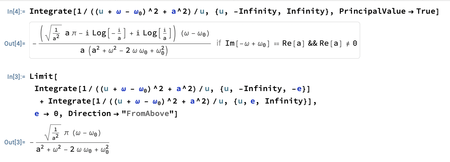
We can’t go any further without figuring out what to do with our nasty little divergent integral \ref{eqn:greensDropWithResistance:220}. We may coerce this into something that we can evaluate using standard contour integration, if we offset the pole at the origin slightly. Given \( \epsilon > 0 \), let’s evaluate
\begin{equation}\label{eqn:greensDropWithResistance:460}
G(\tau, \epsilon) = -\inv{2\pi} \oint \frac{ e^{i z \tau} }{\lr{ z – i \epsilon } \lr{ m z – i \gamma}} dz.
\end{equation}
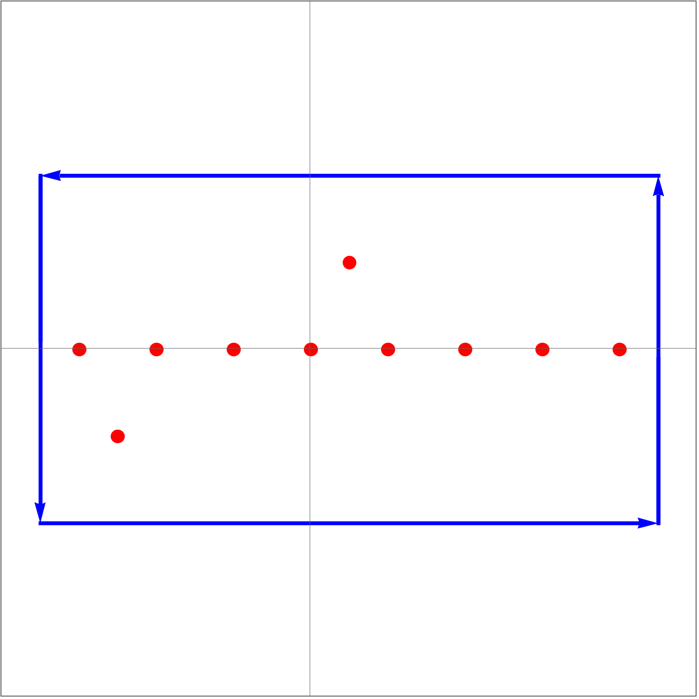
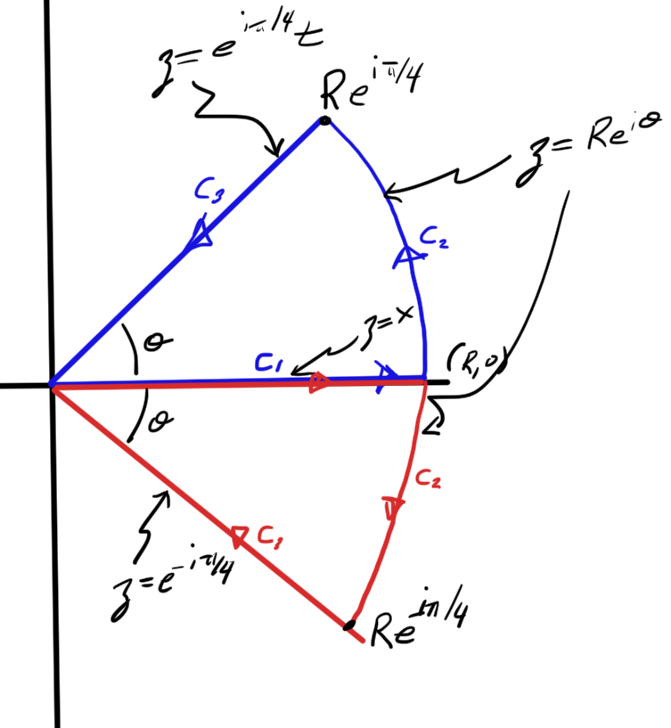
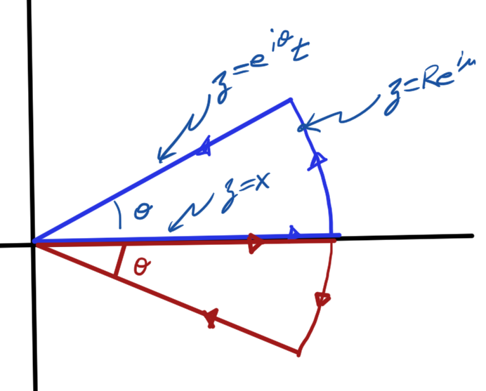
We can evaluate this integral using infinite semicircular contours, using an upper half plane contour for \( \tau > 0 \) and a lower half plane contour for \( \tau < 0 \), as illustrated in fig. 1, and fig. 2.


fig. 1. Contour for tau > 0.


fig. 2. Contour for tau < 0.

By Jordan’s lemma, that upper half plane infinite semicircular part of the contour integral is zero for the \( \tau > 0 \) case, and for the \( \tau < 0 \) case, the lower half plane infinite semicircular part of the contour integral is zero. We can proceed with the residue calculations. In the upper half plane, we have both of the enclosed poles, so \begin{equation}\label{eqn:greensDropWithResistance:480} \begin{aligned} G(\tau > 0, \epsilon)
&= -\inv{2\pi m } \int_{-\infty}^\infty \frac{ e^{i \omega \tau} }{\lr{ \omega – i \epsilon } \lr{ \omega – i \gamma/m}} d\omega \\
&= -\frac{ 2 \pi i }{ 2 \pi m} \lr{
\evalbar{ \frac{ e^{i z \tau} }{ z – i \gamma/m} }{z = i \epsilon}
+
\evalbar{ \frac{ e^{i z \tau} }{ z – i \epsilon } }{ z = i \gamma/m}
} \\
&=
-\frac{i}{m} \lr{
\frac{ e^{-\epsilon \tau} }{ i \epsilon – i \gamma/m}
+
\frac{ e^{-\gamma\tau/m} }{ i \gamma/m – i \epsilon }
} \\
&=
-\lr{
\frac{e^{-\epsilon \tau}}{ m \epsilon – \gamma }
+
\frac{ e^{-\gamma\tau/m} }{ \gamma – m \epsilon }
},
\end{aligned}
\end{equation}
and for the lower half plane, where there are no enclosed poles we have \( G(\tau < 0, \epsilon) = 0 \). In the \( \epsilon \rightarrow 0 \) limit, we are left with
\begin{equation}\label{eqn:greensDropWithResistance:500}
G(\tau) = \inv{\gamma} \lr{ 1 – e^{-\gamma \tau/m} } \Theta(\tau).
\end{equation}

Back to the original problem.

We may now go and find the specific solution for the original problem where \( F(t) = – m g \Be_2 \Theta(t) \). That solution is
\begin{equation}\label{eqn:greensDropWithResistance:520}
\begin{aligned}
\Bx(t)
&= \Bx(0) + \int_{-\infty}^\infty G(t – t’) \lr{ – m g \Be_2 \Theta(t’) } dt’ \\
&= \Bx(0) – m g \Be_2 \int_{-\infty}^\infty \frac{\Theta(t – t’)}{\gamma} \lr{ 1 – e^{-\gamma \lr{ t – t’}/m } } \Theta(t’) dt’ \\
&= \Bx(0) – m g \Be_2 \int_{0}^\infty \frac{\Theta(t – t’)}{\gamma} \lr{ 1 – e^{-\gamma \lr{ t – t’}/m } } dt’ \\
&= \Bx(0) – \frac{m g}{\gamma} \Be_2 \int_{0}^t \lr{ 1 – e^{-\gamma \lr{ t – t’}/m } } dt’ \\
&= \Bx(0) – \frac{m g}{\gamma} \Be_2 \int_0^t \lr{ 1 – e^{-\gamma u/m } } du \\
&= \Bx(0) – \frac{m g}{\gamma} \Be_2 \evalrange{ \lr{ t’ – \frac{e^{-\gamma u/m } }{-\gamma/m} } }{u=0}{t} \\
&= \Bx(0) – \frac{m g}{\gamma} \Be_2 \lr{ t + \frac{m e^{-\gamma t/m }}{\gamma} – \frac{m}{\gamma} } \\
&= \Bx(0) – \frac{m g t}{\gamma} \Be_2 – \frac{m^2 g}{\gamma^2} \lr{ 1 – e^{-\gamma t/m } }.
\end{aligned}
\end{equation}

Ignoring the missing factor of \( g \) on the last term in the twitter slide, this is the final result before the limiting argument on that slide.

Having found the Green’s function for this system, we could then, fairly trivially, use it to solve similar systems with different forcing functions. For example, suppose we have a mass on a table, with friction, and a forcing function (perhaps sinusoidal) moving that mass. We could then figure out the time response for that particular forcing function, and would only have a convolution integral to evaluate. That general applicability is one of the beauties of these transform or Green’s function methods.

A PV integral using contour integration.

January 27, 2025 math and physics play , , , , , ,

[Click here for a PDF version of this post]

Here’s the second last real-integral sub-problem from [1], problem 31(j). Find
\begin{equation}\label{eqn:oscillatorKernel:20}
I = P \int_{-\infty}^\infty \inv{ \lr{ \omega’ – \omega_0 }^2 + a^2 } \inv{ \omega’ – \omega } d\omega’.
\end{equation}

Our poles are sitting at \( \omega \), and
\begin{equation}\label{eqn:oscillatorKernel:80}
\alpha, \beta = \omega_0 \pm i a
\end{equation}
one of which sits above the x-axis, one below, and one on the line.

This means that if we compute the usual infinite semicircular contour integral, we have a \( 2 \pi i \) weighted residue above the line and one \( \pi i \) weighted residue for the x-axis pole. That is
\begin{equation}\label{eqn:oscillatorKernel:50}
\begin{aligned}
\oint \inv{ \lr{ z – \omega_0 }^2 + a^2 } \inv{ z – \omega } dz
&=
\lr{ 2 \pi i } \evalbar{ \inv{\lr{z – \lr{ \omega_0 – i a } } \lr{ z – \omega } } }{z = \omega_0 + i a }
+
\lr{ \pi i } \evalbar{ \inv{ \lr{ z – \omega_0 }^2 + a^2 }}{z = \omega } \\
&=
\lr{ 2 \pi i } \inv{\lr{\omega_0 + i a – \lr{ \omega_0 – i a } } \lr{ \omega_0 + i a – \omega } }
+
\lr{ \pi i } \inv{ \lr{ \omega – \omega_0 }^2 + a^2 } \\
&=
\frac{ 2 \pi i }{2 i a} \inv{ \omega_0 + i a – \omega } \frac{ \omega_0 – i a – \omega }{\omega_0 – i a – \omega }
+
\lr{ \pi i } \inv{ \lr{ \omega – \omega_0 }^2 + a^2 } \\
&=
\frac{ \pi }{ \lr{ \omega – \omega_0 }^2 + a^2 } \lr{ \frac{\omega_0 – \omega}{a} – i + i },
\end{aligned}
\end{equation}
or
\begin{equation}\label{eqn:oscillatorKernel:100}
\boxed{
I =
\frac{ \pi \lr{ \omega_0 – \omega } }{ a \lr{ \lr{ \omega – \omega_0 }^2 + a^2} }.
}
\end{equation}

Interestingly, Mathematica doesn’t seem to be able to solve this integral, even setting PrincipleValue to True. The solution ends up with a bogus seeming \( \textrm{Im}\left(\omega_0-\omega \right) = \textrm{Re}(a) \) restriction, and as far as I can tell, the Mathematica result is also zero after simplification that it fails to do. Mathematica can solve this if we explicitly state the PV condition as a limit, as shown in fig. 1.

fig. 1. Coercing Mathematica to evaluate this.

References

[1] F.W. Byron and R.W. Fuller. Mathematics of Classical and Quantum Physics. Dover Publications, 1992.

A contour integral with a third order pole.

January 21, 2025 math and physics play , , ,

[Click here for a PDF version of this post]

Here’s problem 31(e) from [1]. Find
\begin{equation}\label{eqn:thirdOrderPole:20}
I = \int_0^\infty \frac{x^2 dx}{\lr{ a^2 + x^2 }^3 }.
\end{equation}
Again, we use the contour \( C \) illustrated in fig. 1

fig. 1. Standard above the x-axis, semicircular contour.

Along the infinite semicircle, with \( z = R e^{i\theta} \),
\begin{equation}\label{eqn:thirdOrderPole:40}
\Abs{ \int \frac{z^2 dz}{\lr{ a^2 + z^2 }^3 } } = O(R^3/R^6),
\end{equation}
which tends to zero. We are left to just evaluate some residues
\begin{equation}\label{eqn:thirdOrderPole:60}
\begin{aligned}
I
&= \inv{2} \oint \frac{z^2 dz}{ \lr{ a^2 + z^2 }^3 } \\
&= \inv{2} \oint \frac{z^2 dz}{ \lr{ z – i a }^3 \lr{ z + i a }^3 } \\
&= \inv{2} \lr{ 2 \pi i } \inv{2!} \evalbar{ \frac{d^2}{dz^2} \lr{ \frac{z^2}{ \lr{ z + i a }^3 } } }{z = i a}
\end{aligned}
\end{equation}
Evaluating the derivatives, we have
\begin{equation}\label{eqn:thirdOrderPole:80}
\begin{aligned}
\lr{ \frac{z^2}{ \lr{ z + i a }^3 } }’
&= \frac{ 2 z \lr{ z + i a } – 3 z^2 }{ \lr{ z + i a }^4 } \\
&=
\frac{ – z^2 + 2 i a z }
{ \lr{ z + i a }^4 },
\end{aligned}
\end{equation}
and
\begin{equation}\label{eqn:thirdOrderPole:100}
\begin{aligned}
\frac{d^2}{dz^2} \lr{ \frac{z^2}{ \lr{ z + i a }^3 } }
&= \lr{ \frac{ – z^2 + 2 i a z }
{ \lr{ z + i a }^4 } }’ \\
&= \frac{ \lr{ – 2 z + 2 i a }\lr{ z + i a} – 4 \lr{ – z^2 + 2 i a z }}{ \lr{ z + i a }^5 },
\end{aligned}
\end{equation}
so
\begin{equation}\label{eqn:thirdOrderPole:120}
\begin{aligned}
\evalbar{ \frac{d^2}{dz^2} \lr{ \frac{z^2}{ \lr{ z + i a }^3 } } }{z = i a}
&=
\frac{ \lr{ – 2 i a + 2 i a }\lr{ 2 i a} – 4 \lr{ a^2 – 2 a^2 }}{ \lr{ 2 i a }^5 } \\
&=
\frac{ 4 a^2 }{ \lr{ 2 i a }^5 } \\
&=
\inv{8 a^3 i}.
\end{aligned}
\end{equation}
Putting all the pieces together, we have
\begin{equation}\label{eqn:thirdOrderPole:140}
\boxed{
I = \frac{\pi}{16 a^3}.
}
\end{equation}

References

[1] F.W. Byron and R.W. Fuller. Mathematics of Classical and Quantum Physics. Dover Publications, 1992.

Evaluating a sum using a contour integral.

December 18, 2024 math and physics play , , , , , , , , ,

[Click here for a PDF version of this post]

One of my favorite Dover books, [1], is a powerhouse of a reference, and has a huge set of the mathematical tricks and techniques.  Probably most of the tricks that any engineer or physicist would ever want.

Reading it a bit today, I encountered the following interesting looking theorem for evaluating sums using contour integrals.

Theorem 1.1:

Given a meromorphic function \( f(z) \) that shares no poles with \( \cot( \pi z ) \), where \( C \) encloses the zeros of \( \sin( \pi z \), located at \( z = a, a+1, \cdots b \), then
\begin{equation*}
\sum_{m=a}^b f(m) = \inv{2 \pi i} \oint_C \pi \cot( \pi z ) f(z) dz -\quad \sum_{\mbox{poles of \( f(z) \) in \( C \)}} \mathrm{Res}\lr{ \pi \cot( \pi z ) f(z) }.
\end{equation*}

The enclosing contour may look like fig. 1.

fig. 1. Sample contour

Start proof:

We basically want to evaluate
\begin{equation}\label{eqn:sumUsingContour:20}
\oint_C \pi \cot( \pi z ) f(z) dz,
\end{equation}
using residues. To see why this works, observe that \( \cot( \pi z ) \) is periodic, as plotted in fig. 2.

fig. 2. Cotangent.

In particular, if \( z = m + \epsilon \), we have
\begin{equation}\label{eqn:sumUsingContour:40}
\begin{aligned}
\cot(\pi z)
&= \frac{\cos(\pi(m + \epsilon))}{\sin(\pi(m + \epsilon))} \\
&= \frac{(-1)^m \cos(\pi \epsilon)}{(-1)^m \sin(\pi \epsilon)} \\
&= \cot(\pi \epsilon).
\end{aligned}
\end{equation}
The residue of \( \pi \cot(\pi z) \), at \( z = 0 \), or at any other integer point, is
\begin{equation}\label{eqn:sumUsingContour:60}
\frac{\pi}{
\pi z – (\pi z)^3/6 + \cdots
}
= 1.
\end{equation}
This means that we have
\begin{equation}\label{eqn:sumUsingContour:80}
\oint_C \pi \cot( \pi z ) f(z) dz = 2 \pi i \sum_{m = a}^b f(m) + 2 \pi i \quad \sum_{\mbox{poles of \( f(z) \) in \( C \)}} \mathrm{Res}\lr{ \pi \cot( \pi z ) f(z) }.
\end{equation}
We just have to rearrange and scale to complete the proof.

End proof.

In the book the sample application was to use this to show that
\begin{equation}\label{eqn:sumUsingContour:100}
\coth x – \inv{x} = \sum_{m=1}^\infty \frac{2x}{x^2 + m^2 \pi^2}.
\end{equation}
That’s then integrated to show that
\begin{equation}\label{eqn:sumUsingContour:120}
\frac{\sinh x}{x} = \prod_{m = 1}^\infty \lr{ 1 + \frac{x^2}{m^2 \pi^2} },
\end{equation}
or with \( x = i \theta \),
\begin{equation}\label{eqn:sumUsingContour:140}
\sin \theta = \theta \prod_{m = 1}^\infty \lr{ 1 – \frac{\theta^2}{m^2 \pi^2} },
\end{equation}
and finally equating \( \theta^3 \) terms in this infinite product, we find
\begin{equation}\label{eqn:sumUsingContour:160}
\sum_{m = 1}^\infty \inv{m^2} = \frac{\pi^2}{6},
\end{equation}
which is \( \zeta(2) \), a specific value of the Riemann zeta function.

All this is done in a couple spectacularly dense pages of calculation, and illustrates the kind of gems in this book. At about 700 pages, it’s got a lot of gems.

References

[1] F.W. Byron and R.W. Fuller. Mathematics of Classical and Quantum Physics. Dover Publications, 1992.

Generalized Gaussian integrals

September 10, 2015 phy1520 , , , ,

[Click here for a PDF of this post with nicer formatting]

Both [3] and [4] use Gaussian integrals with both (negative) real, and imaginary arguments, which give the impression that the following is true:

\begin{equation}\label{eqn:generalizedGaussian:20}
\int_{-\infty}^\infty \exp\lr{ a x^2 } dx = \sqrt{\frac{-\pi}{a}},
\end{equation}

even when \( a \) is not a real negative constant, and in particular, with values \( a = \pm i \). Clearly this doesn’t follow by just making a substition \( x \rightarrow x/\sqrt{a} \), since that moves the integration range onto a rotated path in the complex plane when \( a \) is \( \pm i \). However, with some care, it can be shown that \ref{eqn:generalizedGaussian:20} holds provided \( \textrm{Re} \, a \le 0 \).

The first special case is \( \int_{-\infty}^\infty \exp\lr{ – x^2 } dx = \sqrt{\pi} \) which is easy to derive using the usual square it and integrate in circular coordinates trick.

Purely imaginary cases.

Let’s handle the \( a = \pm i \) cases next. These can be evaluated by considering integrals over the contours of fig. 1, where the upper plane contour is used for \( a = i \) and the lower plane contour for \( a = -i \).

twoContours45DegreesFig1

fig. 1. Contours for a = i,-i

Since there are no poles, the integral over either such contour is zero. Credit for figuring out how to tackle that integral and what contour to use goes to Dr MV, on stackexchange [2].

For the upper plane contour we have

\begin{equation}\label{eqn:generalizedGaussian:40}
\begin{aligned}
0
&= \oint \exp\lr{ i z^2 } dz \\
&= \int_0^R \exp\lr{ i x^2 } dx
+ \int_0^{\pi/4} \exp\lr{ i R^2 e^{2 i \theta} } R i e^{i\theta} d\theta
+ \int_R^0 \exp\lr{ i^2 t^2 } e^{i\pi/4} dt.
\end{aligned}
\end{equation}

Observe that \( i e^{2 i \theta} = i\cos(2 \theta) – \sin(2\theta) \) which has a negative real part for all values of \( \theta \ne 0 \). Provided the contour is slightly deformed from the axis, that second integral has a term of the form \( \sim R e^{-R^2} \) which tends to zero as \( R \rightarrow \infty \). So in the limit, this is

\begin{equation}\label{eqn:generalizedGaussian:60}
\int_0^\infty \exp\lr{ i x^2 } dx
= \sqrt{\pi} e^{i\pi/4}/2,
\end{equation}

or
\begin{equation}\label{eqn:generalizedGaussian:80}
\int_{-\infty}^\infty \exp\lr{ i x^2 } dx
= \sqrt{i \pi},
\end{equation}

a special case of \ref{eqn:generalizedGaussian:20} as desired. For \( a = -i \) integrating around the lower plane contour, we have

\begin{equation}\label{eqn:generalizedGaussian:100}
\begin{aligned}
0
&= \oint \exp\lr{ -i z^2 } dz \\
&= \int_0^R \exp\lr{ i x^2 } dx
+ \int_0^{-\pi/4} \exp\lr{ -i R^2 e^{2 i \theta} } R i e^{i\theta} d\theta
+ \int_R^0 \exp\lr{ -i (-i) t^2 } e^{-i\pi/4} dt.
\end{aligned}
\end{equation}

This time, in the second integral we also have \( -i R^2 e^{2 i \theta} = i R^2 \cos(2 \theta) + \sin(2 \theta) \), which also has a negative real part for \( \theta \in (0, \pi/4] \). Again the contour needs to be infinitesimally deformed, placed just lower than the axis.

This time we find

\begin{equation}\label{eqn:generalizedGaussian:120}
\int_{-\infty}^\infty \exp\lr{ -i x^2 } dx
= \sqrt{-i \pi},
\end{equation}

another special case of \ref{eqn:generalizedGaussian:20}.

Note.

Distorting the contour in this fashion seems somewhat like handwaving. A better approach would probably follow [1] where Jordan’s lemma is covered. It doesn’t look like Jordan’s lemma applies as is to this case, but the arguments look like they could be adapted appropriately.

Completely complex case.

A similar trick can be used to evaluate the more general cases, but a bit of thought is required to figure out the contours required. More precisely, while these contours will still have a wedge of pie shape, as sketched in fig. 2, we have to figure out the angle subtended by the edge of this piece of pie.

twoContoursThetaFig2

fig. 2. Contours for complex a.

To evaluate an integral consider

\begin{equation}\label{eqn:generalizedGaussian:140}
\begin{aligned}
0
&= \oint \exp\lr{ e^{i\phi} z^2 } dz \\
&= \int_0^R \exp\lr{ e^{i\phi} x^2 } dx
+ \int_0^{\theta} \exp\lr{ e^{i\phi} R^2 e^{2 i \mu} } R i e^{i\mu} d\mu
+ \int_R^0 \exp\lr{ e^{i\phi} e^{2 i \theta} t^2 } e^{i\theta} dt,
\end{aligned}
\end{equation}

where \( \phi \in (\pi/2, \pi) \cup (\pi,3\pi/2) \). We have a hope of evaluating this last integral if \( \phi + 2 \theta = \pi \), or

\begin{equation}\label{eqn:generalizedGaussian:160}
\theta = (\pi -\phi)/2,
\end{equation}

giving

\begin{equation}\label{eqn:generalizedGaussian:180}
\int_0^R \exp\lr{ e^{i\phi} x^2 } dx
=
e^{i\lr{\pi – \phi}/2} \int_0^R \exp\lr{ -t^2 } dt
– \int_0^{\theta} \exp\lr{ R^2 \lr{ \cos\lr{\phi + 2 \mu} + i \sin\lr{\phi + 2 \mu}} } R i e^{i\mu} d\mu.
\end{equation}

If the cosine is always negative on the chosen contours, then that integral will vanish in the \( R \rightarrow \infty \) limit. This turns out to be the case, which can be confirmed by considering each of the contours in sequence. If the upper plane contour is used to evaluate the integral for the \( \phi \in (\pi/2,\pi) \) case, we have

\begin{equation}\label{eqn:generalizedGaussian:200}
\theta \in (0, \pi/4).
\end{equation}

Since \( \phi + 2\theta = \pi \), we have

\begin{equation}\label{eqn:generalizedGaussian:220}
\phi + 2 \mu \in (\pi/2, \pi),
\end{equation}

and find that the cosine is strictly negative on that contour for that range of \( \phi \). Picking the lower plane contour for the \( \phi \in (\pi, 3\pi/2) \) range, we have

\begin{equation}\label{eqn:generalizedGaussian:240}
\theta \in (-\pi/4, 0),
\end{equation}

and so

\begin{equation}\label{eqn:generalizedGaussian:260}
\phi + 2 \mu \in (\pi/2, 3\pi/2).
\end{equation}

For this range of \( \phi \) the cosine on the lower plane contour is again negative as desired, so in the infinite \( R \) limit we have

\begin{equation}\label{eqn:generalizedGaussian:280}
\int_0^\infty \exp\lr{ e^{i\phi} x^2 } dx
=
\inv{2} \sqrt{ -\pi e^{-i\phi} }.
\end{equation}

The points at \( \phi = \pi/2, \pi, 3\pi/2 \) were omitted, but we’ve found the same result at those points, completing the verification of \ref{eqn:generalizedGaussian:20} for all \( \textrm{Re} a \le 0 \).

References

[1] W.R. Le Page and W.R. LePage. Complex Variables and the Laplace Transform for Engineers, chapter 8-10. A Theorem for Trigonometric Integrals. Courier Dover Publications, 1980.

[2] Dr. MV. Evaluating definite integral of exp(i t^2), 2015. URL https://math.stackexchange.com/a/1411084/359. [Online; accessed 10-September-2015].

[3] Jun John Sakurai and Jim J Napolitano. Modern quantum mechanics. Pearson Higher Ed, 2014.

[4] A. Zee. Quantum field theory in a nutshell. Universities Press, 2005.