convex optimization

ECE1505H Convex Optimization. Lecture 8: Local vs. Global, and composition of functions. Taught by Prof. Stark Draper

February 4, 2017 ece1505 , , , ,

[Click here for a PDF of this post with nicer formatting]

Disclaimer

Peeter’s lecture notes from class. These may be incoherent and rough.

These are notes for the UofT course ECE1505H, Convex Optimization, taught by Prof. Stark Draper, from [1].

Today

  • Finish local vs global.
  • Compositions of functions.
  • Introduction to convex optimization problems.

Continuing proof:

We want to prove that if

\begin{equation*}
\begin{aligned}
\spacegrad F(\Bx^\conj) &= 0 \\
\spacegrad^2 F(\Bx^\conj) \ge 0
\end{aligned},
\end{equation*}

then \( \Bx^\conj\) is a local optimum.

Proof:

Again, using Taylor approximation

\begin{equation}\label{eqn:convexOptimizationLecture8:20}
F(\Bx^\conj + \Bv) = F(\Bx^\conj) + \lr{ \spacegrad F(\Bx^\conj)}^\T \Bv + \inv{2} \Bv^\T \spacegrad^2 F(\Bx^\conj) \Bv + o(\Norm{\Bv}^2)
\end{equation}

The linear term is zero by assumption, whereas the Hessian term is given as \( > 0 \). Any direction that you move in, if your move is small enough, this is going uphill at a local optimum.

Summarize:

For twice continuously differentiable functions, at a local optimum \( \Bx^\conj \), then

\begin{equation}\label{eqn:convexOptimizationLecture8:40}
\begin{aligned}
\spacegrad F(\Bx^\conj) &= 0 \\
\spacegrad^2 F(\Bx^\conj) \ge 0
\end{aligned}
\end{equation}

If, in addition, \( F \) is convex, then \( \spacegrad F(\Bx^\conj) = 0 \) implies that \( \Bx^\conj \) is a global optimum. i.e. for (unconstrained) convex functions, local and global optimums are equivalent.

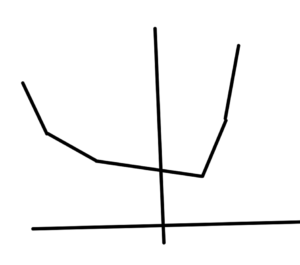
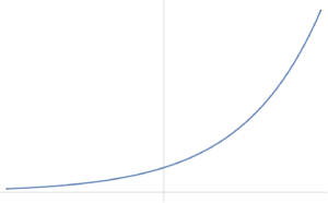
  • It is possible that a convex function does not have a global optimum. Examples are \( F(x) = e^x \)
    (fig. 1)
    , which has an \( \inf \), but no lowest point.

    fig. 1. Exponential has no global optimum.

  • Our discussion has been for unconstrained functions. For constrained problems (next topic) is not not necessarily true that \( \spacegrad F(\Bx) = 0 \) implies that \( \Bx \) is a global optimum, even for \( F \) convex.

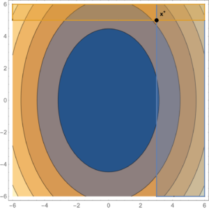
    As an example of a constrained problem consider

    \begin{equation}\label{eqn:convexOptimizationLecture8:n}
    \begin{aligned}
    \min &2 x^2 + y^2 \\
    x &\ge 3 \\
    y &\ge 5.
    \end{aligned}
    \end{equation}

    The level sets of this objective function are plotted in fig. 2. The optimal point is at \( \Bx^\conj = (3,5) \), where \( \spacegrad F \ne 0 \).

    fig. 2. Constrained problem with optimum not at the zero gradient point.

Projection

Given \( \Bx \in \mathbb{R}^n, \By \in \mathbb{R}^p \), if \( h(\Bx,\By) \) is convex in \( \Bx, \By \), then

\begin{equation}\label{eqn:convexOptimizationLecture8:60}
F(\Bx_0) = \inf_\By h(\Bx_0,\By)
\end{equation}

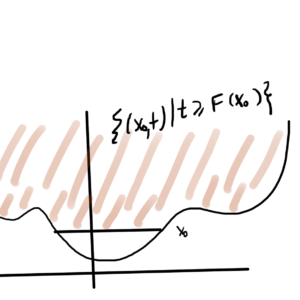
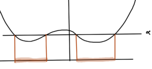
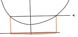
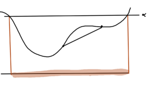
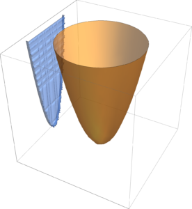
is convex in \( \Bx\), as sketched in fig. 3.

fig. 3. Epigraph of \( h \) is a filled bowl.

The intuition here is that shining light on the (filled) “bowl”. That is, the image of \( \textrm{epi} h \) on the \( \By = 0 \) screen which we will show is a convex set.

Proof:

Since \( h \) is convex in \( \begin{bmatrix} \Bx \\ \By \end{bmatrix} \in \textrm{dom} h \), then

\begin{equation}\label{eqn:convexOptimizationLecture8:80}
\textrm{epi} h = \setlr{ (\Bx,\By,t) | t \ge h(\Bx,\By), \begin{bmatrix} \Bx \\ \By \end{bmatrix} \in \textrm{dom} h },
\end{equation}

is a convex set.

We also have to show that the domain of \( F \) is a convex set. To show this note that

\begin{equation}\label{eqn:convexOptimizationLecture8:100}
\begin{aligned}
\textrm{dom} F
&= \setlr{ \Bx | \exists \By s.t. \begin{bmatrix} \Bx \\ \By \end{bmatrix} \in \textrm{dom} h } \\
&= \setlr{
\begin{bmatrix}
I_{n\times n} & 0_{n \times p}
\end{bmatrix}
\begin{bmatrix}
\Bx \\
\By
\end{bmatrix}
| \begin{bmatrix} \Bx \\ \By \end{bmatrix} \in \textrm{dom} h
}.
\end{aligned}
\end{equation}

This is an affine map of a convex set. Therefore \( \textrm{dom} F \) is a convex set.

\begin{equation}\label{eqn:convexOptimizationLecture8:120}
\begin{aligned}
\textrm{epi} F
&=
\setlr{ \begin{bmatrix} \Bx \\ \By \end{bmatrix} | t \ge \inf h(\Bx,\By), \Bx \in \textrm{dom} F, \By: \begin{bmatrix} \Bx \\ \By \end{bmatrix} \in \textrm{dom} h } \\
&=
\setlr{
\begin{bmatrix}
I & 0 & 0 \\
0 & 0 & 1
\end{bmatrix}
\begin{bmatrix}
\Bx \\
\By \\
t
\end{bmatrix}
|
t \ge h(\Bx,\By), \begin{bmatrix} \Bx \\ \By \end{bmatrix} \in \textrm{dom} h
}.
\end{aligned}
\end{equation}

Example:

The function

\begin{equation}\label{eqn:convexOptimizationLecture8:140}
F(\Bx) = \inf_{\By \in C} \Norm{ \Bx – \By },
\end{equation}

over \( \Bx \in \mathbb{R}^n, \By \in C \), ,is convex if \( C \) is a convex set. Reason:

  • \( \Bx – \By \) is linear in \((\Bx, \By)\).
  • \( \Norm{ \Bx – \By } \) is a convex function if the domain is a convex set
  • The domain is \( \mathbb{R}^n \times C \). This will be a convex set if \( C \) is.
  • \( h(\Bx, \By) = \Norm{\Bx -\By} \) is a convex function if \( \textrm{dom} h \) is a convex set. By setting \( \textrm{dom} h = \mathbb{R}^n \times C \), if \( C \) is convex, \( \textrm{dom} h \) is a convex set.
  • \( F() \)

Composition of functions

Consider

\begin{equation}\label{eqn:convexOptimizationLecture8:160}
\begin{aligned}
F(\Bx) &= h(g(\Bx)) \\
\textrm{dom} F &= \setlr{ \Bx \in \textrm{dom} g | g(\Bx) \in \textrm{dom} h } \\
F &: \mathbb{R}^n \rightarrow \mathbb{R} \\
g &: \mathbb{R}^n \rightarrow \mathbb{R} \\
h &: \mathbb{R} \rightarrow \mathbb{R}.
\end{aligned}
\end{equation}

Cases:

  1. \( g \) is convex, \( h \) is convex and non-decreasing.
  2. \( g \) is convex, \( h \) is convex and non-increasing.

Show for 1D case ( \( n = 1 \)). Get to \( n > 1 \) by applying to all lines.

  1. \begin{equation}\label{eqn:convexOptimizationLecture8:180}
    \begin{aligned}
    F'(x) &= h'(g(x)) g'(x) \\
    F”(x) &=
    h”(g(x)) g'(x) g'(x)
    +
    h'(g(x)) g”(x) \\
    &=
    h”(g(x)) (g'(x))^2
    +
    h'(g(x)) g”(x) \\
    &=
    \lr{ \ge 0 } \cdot \lr{ \ge 0 }^2 + \lr{ \ge 0 } \cdot \lr{ \ge 0 },
    \end{aligned}
    \end{equation}

    since \( h \) is respectively convex, and non-decreasing.

  2. \begin{equation}\label{eqn:convexOptimizationLecture8:180b}
    \begin{aligned}
    F'(x) =
    \lr{ \ge 0 } \cdot \lr{ \ge 0 }^2 + \lr{ \le 0 } \cdot \lr{ \le 0 },
    \end{aligned}
    \end{equation}

    since \( h \) is respectively convex, and non-increasing, and g is concave.

Extending to multiple dimensions

\begin{equation}\label{eqn:convexOptimizationLecture8:200}
\begin{aligned}
F(\Bx)
&= h(g(\Bx)) = h( g_1(\Bx), g_2(\Bx), \cdots g_k(\Bx) ) \\
g &: \mathbb{R}^n \rightarrow \mathbb{R} \\
h &: \mathbb{R}^k \rightarrow \mathbb{R}.
\end{aligned}
\end{equation}

is convex if \( g_i \) is convex for each \( i \in [1,k] \) and \( h \) is convex and non-decreasing in each argument.

Proof:

again assume \( n = 1 \), without loss of generality,

\begin{equation}\label{eqn:convexOptimizationLecture8:220}
\begin{aligned}
g &: \mathbb{R} \rightarrow \mathbb{R}^k \\
h &: \mathbb{R}^k \rightarrow \mathbb{R} \\
\end{aligned}
\end{equation}

\begin{equation}\label{eqn:convexOptimizationLecture8:240}
F”(\Bx)
=
\begin{bmatrix}
g_1(\Bx) & g_2(\Bx) & \cdots & g_k(\Bx)
\end{bmatrix}
\spacegrad^2 h(g(\Bx))
\begin{bmatrix}
g_1′(\Bx) \\ g_2′(\Bx) \\ \vdots \\ g_k'(\Bx)
\end{bmatrix}
+
\lr{ \spacegrad h(g(x)) }^\T
\begin{bmatrix}
g_1”(\Bx) \\ g_2”(\Bx) \\ \vdots \\ g_k”(\Bx)
\end{bmatrix}
\end{equation}

The Hessian is PSD.

Example:

\begin{equation}\label{eqn:convexOptimizationLecture8:260}
F(x) = \exp( g(x) ) = h( g(x) ),
\end{equation}

where \( g \) is convex is convex, and \( h(y) = e^y \). This implies that \( F \) is a convex function.

Example:

\begin{equation}\label{eqn:convexOptimizationLecture8:280}
F(x) = \inv{g(x)},
\end{equation}

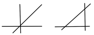
is convex if \( g(x) \) is concave and positive. The most simple such example of such a function is \( h(x) = 1/x, \textrm{dom} h = \mathbb{R}_{++} \), which is plotted in fig. 4.

fig. 4. Inverse function is convex over positive domain.

Example:

\begin{equation}\label{eqn:convexOptimizationLecture8:300}
F(x) = – \sum_{i = 1}^n \log( -F_i(x) )
\end{equation}

is convex on \( \setlr{ x | F_i(x) < 0 \forall i } \) if all \( F_i \) are convex.

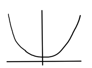
  • Due to \( \textrm{dom} F \), \( -F_i(x) > 0 \,\forall x \in \textrm{dom} F \)
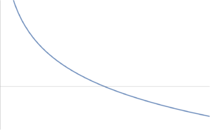
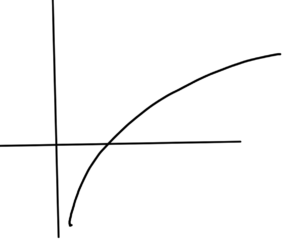
  • \( \log(x) \) concave on \( \mathbb{R}_{++} \) so \( -\log \) convex also non-increasing (fig. 5).

    fig. 5. Negative logarithm convex over positive domain.

\begin{equation}\label{eqn:convexOptimizationLecture8:320}
F(x) = \sum h_i(x)
\end{equation}

but
\begin{equation}\label{eqn:convexOptimizationLecture8:340}
h_i(x) = -\log(-F_i(x)),
\end{equation}

which is a convex and non-increasing function (\(-\log\)), of a convex function \( -F_i(x) \). Each
\( h_i \) is convex, so this is a sum of convex functions, and is therefore convex.

Example:

Over \( \textrm{dom} F = S^n_{++} \)

\begin{equation}\label{eqn:convexOptimizationLecture8:360}
F(X) = \log \det X^{-1}
\end{equation}

To show that this is convex, check all lines in domain. A line in \( S^n_{++} \) is a 1D family of matrices

\begin{equation}\label{eqn:convexOptimizationLecture8:380}
\tilde{F}(t) = \log \det( \lr{X_0 + t H}^{-1} ),
\end{equation}

where \( X_0 \in S^n_{++}, t \in \mathbb{R}, H \in S^n \).

F9

For \( t \) small enough,

\begin{equation}\label{eqn:convexOptimizationLecture8:400}
X_0 + t H \in S^n_{++}
\end{equation}

\begin{equation}\label{eqn:convexOptimizationLecture8:420}
\begin{aligned}
\tilde{F}(t)
&= \log \det( \lr{X_0 + t H}^{-1} ) \\
&= \log \det\lr{ X_0^{-1/2} \lr{I + t X_0^{-1/2} H X_0^{-1/2} }^{-1} X_0^{-1/2} } \\
&= \log \det\lr{ X_0^{-1} \lr{I + t X_0^{-1/2} H X_0^{-1/2} }^{-1} } \\
&= \log \det X_0^{-1} + \log\det \lr{I + t X_0^{-1/2} H X_0^{-1/2} }^{-1} \\
&= \log \det X_0^{-1} – \log\det \lr{I + t X_0^{-1/2} H X_0^{-1/2} } \\
&= \log \det X_0^{-1} – \log\det \lr{I + t M }.
\end{aligned}
\end{equation}

If \( \lambda_i \) are eigenvalues of \( M \), then \( 1 + t \lambda_i \) are eigenvalues of \( I + t M \). i.e.:

\begin{equation}\label{eqn:convexOptimizationLecture8:440}
\begin{aligned}
(I + t M) \Bv
&=
I \Bv + t \lambda_i \Bv \\
&=
(1 + t \lambda_i) \Bv.
\end{aligned}
\end{equation}

This gives

\begin{equation}\label{eqn:convexOptimizationLecture8:460}
\begin{aligned}
\tilde{F}(t)
&= \log \det X_0^{-1} – \log \prod_{i = 1}^n (1 + t \lambda_i) \\
&= \log \det X_0^{-1} – \sum_{i = 1}^n \log (1 + t \lambda_i)
\end{aligned}
\end{equation}

  • \( 1 + t \lambda_i \) is linear in \( t \).
  • \( -\log \) is convex in its argument.
  • sum of convex function is convex.

Example:

\begin{equation}\label{eqn:convexOptimizationLecture8:480}
F(X) = \lambda_\max(X),
\end{equation}

is convex on \( \textrm{dom} F \in S^n \)

(a)
\begin{equation}\label{eqn:convexOptimizationLecture8:500}
\lambda_{\max} (X) = \sup_{\Norm{\Bv}_2 \le 1} \Bv^\T X \Bv,
\end{equation}

\begin{equation}\label{eqn:convexOptimizationLecture8:520}
\begin{bmatrix}
\lambda_1 & & & \\
& \lambda_2 & & \\
& & \ddots & \\
& & & \lambda_n
\end{bmatrix}
\end{equation}

Recall that a decomposition

\begin{equation}\label{eqn:convexOptimizationLecture8:540}
\begin{aligned}
X &= Q \Lambda Q^\T \\
Q^\T Q = Q Q^\T = I
\end{aligned}
\end{equation}

can be used for any \( X \in S^n \).

(b)

Note that \( \Bv^\T X \Bv \) is linear in \( X \). This is a max of a number of linear (and convex) functions, so it is convex.

Last example:

(non-symmetric matrices)

\begin{equation}\label{eqn:convexOptimizationLecture8:560}
F(X) = \sigma_\max(X),
\end{equation}

is convex on \( \textrm{dom} F = \mathbb{R}^{m \times n} \). Here

\begin{equation}\label{eqn:convexOptimizationLecture8:580}
\sigma_\max(X) = \sup_{\Norm{\Bv}_2 = 1} \Norm{X \Bv}_2
\end{equation}

This is called an operator norm of \( X \). Using the SVD

\begin{equation}\label{eqn:convexOptimizationLecture8:600}
\begin{aligned}
X &= U sectionigma V^\T \\
U &= \mathbb{R}^{m \times r} \\
sectionigma &\in \mathrm{diag} \in \mathbb{R}{ r \times r } \\
V^T &\in \mathbb{R}^{r \times n}.
\end{aligned}
\end{equation}

Have

\begin{equation}\label{eqn:convexOptimizationLecture8:620}
\Norm{X \Bv}_2^2
=
\Norm{ U sectionigma V^\T \Bv }_2^2
=
\Bv^\T V sectionigma U^\T U sectionigma V^\T \Bv
=
\Bv^\T V sectionigma sectionigma V^\T \Bv
=
\Bv^\T V sectionigma^2 V^\T \Bv
=
\tilde{\Bv}^\T sectionigma^2 \tilde{\Bv},
\end{equation}

where \( \tilde{\Bv} = \Bv^\T V \), so

\begin{equation}\label{eqn:convexOptimizationLecture8:640}
\Norm{X \Bv}_2^2
=
\sum_{i = 1}^r \sigma_i^2 \Norm{\tilde{\Bv}}
\le \sigma_\max^2 \Norm{\tilde{\Bv}}^2,
\end{equation}

or
\begin{equation}\label{eqn:convexOptimizationLecture8:660}
\Norm{X \Bv}_2
\le \sqrt{ \sigma_\max^2 } \Norm{\tilde{\Bv}}
\le
\sigma_\max.
\end{equation}

Set \( \Bv \) to the right singular value of \( X \) to get equality.

References

[1] Stephen Boyd and Lieven Vandenberghe. Convex optimization. Cambridge university press, 2004.
ECE1505H Convex Optimization. Lecture 7: Examples of convex and concave functions, local and global minimums. Taught by Prof. Stark Draper

February 2, 2017 Uncategorized , , , , , , ,

[Click here for a PDF of this post with nicer formatting]

Disclaimer

Peeter’s lecture notes from class. These may be incoherent and rough.

These are notes for the UofT course ECE1505H, Convex Optimization, taught by Prof. Stark Draper, from [1].

Today

  • Local and global optimality
  • Compositions of functions
  • Examples

Example:

\begin{equation}\label{eqn:convexOptimizationLecture7:20}
\begin{aligned}
F(x) &= x^2 \\
F”(x) &= 2 > 0
\end{aligned}
\end{equation}

strictly convex.

Example:

\begin{equation}\label{eqn:convexOptimizationLecture7:40}
\begin{aligned}
F(x) &= x^3 \\
F”(x) &= 6 x.
\end{aligned}
\end{equation}

Not always non-negative, so not convex. However \( x^3 \) is convex on \( \textrm{dom} F = \mathbb{R}_{+} \).

Example:

\begin{equation}\label{eqn:convexOptimizationLecture7:60}
\begin{aligned}
F(x) &= x^\alpha \\
F'(x) &= \alpha x^{\alpha-1} \\
F”(x) &= \alpha(\alpha-1) x^{\alpha-2}.
\end{aligned}
\end{equation}


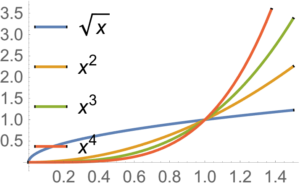
fig. 1. Powers of x.

This is convex on \( \mathbb{R}_{+} \), if \( \alpha \ge 1 \), or \( \alpha \le 0 \).

Example:

\begin{equation}\label{eqn:convexOptimizationLecture7:80}
\begin{aligned}
F(x) &= \log x \\
F'(x) &= \inv{x} \\
F”(x) &= -\inv{x^2} \le 0
\end{aligned}
\end{equation}

This is concave.

Example:

\begin{equation}\label{eqn:convexOptimizationLecture7:100}
\begin{aligned}
F(x) &= x\log x \\
F'(x) &= \log x + x \inv{x} = 1 + \log x \\
F”(x) &= \inv{x}
\end{aligned}
\end{equation}

This is strictly convex on
\( \mathbb{R}_{++} \), where
\( F”(x) \ge 0 \).

Example:

\begin{equation}\label{eqn:convexOptimizationLecture7:120}
\begin{aligned}
F(x) &= e^{\alpha x} \\
F'(x) &= \alpha e^{\alpha x} \\
F”(x) &= \alpha^2 e^{\alpha x} \ge 0
\end{aligned}
\end{equation}

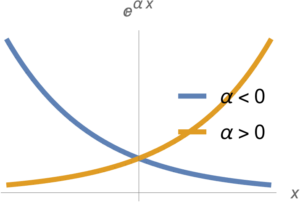
fig. 2. Exponential.

Such functions are plotted in fig. 2, and are convex function for all \( \alpha \).

Example:

For symmetric \( P \in S^n \)

\begin{equation}\label{eqn:convexOptimizationLecture7:140}
\begin{aligned}
F(\Bx) &= \Bx^\T P \Bx + 2 \Bq^\T \Bx + r \\
\spacegrad F &= (P + P^\T) \Bx + 2 \Bq = 2 P \Bx + 2 \Bq \\
\spacegrad^2 F &= 2 P.
\end{aligned}
\end{equation}

This is convex(concave) if \( P \ge 0 \) (\( P \le 0\)).

Example:

A quadratic function

\begin{equation}\label{eqn:convexOptimizationLecture7:780}
F(x, y) = x^2 + y^2 + 3 x y,
\end{equation}

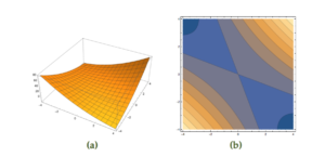
that is neither convex nor concave is plotted in fig 3.

fig 3. Function with saddle point (3d and contours)

This function can be put in matrix form

\begin{equation}\label{eqn:convexOptimizationLecture7:160}
F(x, y) = x^2 + y^2 + 3 x y
=
\begin{bmatrix}
x & y
\end{bmatrix}
\begin{bmatrix}
1 & 1.5 \\
1.5 & 1
\end{bmatrix}
\begin{bmatrix}
x \\
y
\end{bmatrix},
\end{equation}

and has the Hessian

\begin{equation}\label{eqn:convexOptimizationLecture7:180}
\begin{aligned}
\spacegrad^2 F
&=
\begin{bmatrix}
\partial_{xx} F & \partial_{xy} F \\
\partial_{yx} F & \partial_{yy} F \\
\end{bmatrix} \\
&=
\begin{bmatrix}
2 & 3 \\
3 & 2
\end{bmatrix} \\
&= 2 P.
\end{aligned}
\end{equation}

From the plot we know that this is not PSD, but this can be confirmed by checking the eigenvalues

\begin{equation}\label{eqn:convexOptimizationLecture7:200}
\begin{aligned}
0
&=
\det ( P – \lambda I ) \\
&=
(1 – \lambda)^2 – 1.5^2,
\end{aligned}
\end{equation}

which has solutions

\begin{equation}\label{eqn:convexOptimizationLecture7:220}
\lambda = 1 \pm \frac{3}{2} = \frac{3}{2}, -\frac{1}{2}.
\end{equation}

This is not PSD nor negative semi-definite, because it has one positive and one negative eigenvalues. This is neither convex nor concave.

Along \( y = -x \),

\begin{equation}\label{eqn:convexOptimizationLecture7:240}
\begin{aligned}
F(x,y)
&=
F(x,-x) \\
&=
2 x^2 – 3 x^2 \\
&=
– x^2,
\end{aligned}
\end{equation}

so it is concave along this line. Along \( y = x \)

\begin{equation}\label{eqn:convexOptimizationLecture7:260}
\begin{aligned}
F(x,y)
&=
F(x,x) \\
&=
2 x^2 + 3 x^2 \\
&=
5 x^2,
\end{aligned}
\end{equation}

so it is convex along this line.

Example:

\begin{equation}\label{eqn:convexOptimizationLecture7:280}
F(\Bx) = \sqrt{ x_1 x_2 },
\end{equation}

on \( \textrm{dom} F = \setlr{ x_1 \ge 0, x_2 \ge 0 } \)

For the Hessian
\begin{equation}\label{eqn:convexOptimizationLecture7:300}
\begin{aligned}
\PD{x_1}{F} &= \frac{1}{2} x_1^{-1/2} x_2^{1/2} \\
\PD{x_2}{F} &= \frac{1}{2} x_2^{-1/2} x_1^{1/2}
\end{aligned}
\end{equation}

The Hessian components are

\begin{equation}\label{eqn:convexOptimizationLecture7:320}
\begin{aligned}
\PD{x_1}{} \PD{x_1}{F} &= -\frac{1}{4} x_1^{-3/2} x_2^{1/2} \\
\PD{x_1}{} \PD{x_2}{F} &= \frac{1}{4} x_2^{-1/2} x_1^{-1/2} \\
\PD{x_2}{} \PD{x_1}{F} &= \frac{1}{4} x_1^{-1/2} x_2^{-1/2} \\
\PD{x_2}{} \PD{x_2}{F} &= -\frac{1}{4} x_2^{-3/2} x_1^{1/2}
\end{aligned}
\end{equation}

or
\begin{equation}\label{eqn:convexOptimizationLecture7:340}
\spacegrad^2 F
=
-\frac{\sqrt{x_1 x_2}}{4}
\begin{bmatrix}
\inv{x_1^2} & -\inv{x_1 x_2} \\
-\inv{x_1 x_2} & \inv{x_2^2}
\end{bmatrix}.
\end{equation}

Checking this for PSD against \( \Bv = (v_1, v_2) \), we have
\begin{equation}\label{eqn:convexOptimizationLecture7:360}
\begin{aligned}
\begin{bmatrix}
v_1 & v_2
\end{bmatrix}
\begin{bmatrix}
\inv{x_1^2} & -\inv{x_1 x_2} \\
-\inv{x_1 x_2} & \inv{x_2^2}
\end{bmatrix}
\begin{bmatrix}
v_1 \\ v_2
\end{bmatrix}
&=
\begin{bmatrix}
v_1 & v_2
\end{bmatrix}
\begin{bmatrix}
\inv{x_1^2} v_1 -\inv{x_1 x_2} v_2 \\
-\inv{x_1 x_2} v_1 + \inv{x_2^2} v_2
\end{bmatrix} \\
&=
\lr{ \inv{x_1^2} v_1 -\inv{x_1 x_2} v_2 } v_1 +
\lr{ -\inv{x_1 x_2} v_1 + \inv{x_2^2} v_2 } v_2
\\
&=
\inv{x_1^2} v_1^2
+ \inv{x_2^2} v_2^2
-2 \inv{x_1 x_2} v_1 v_2 \\
&=
\lr{
\frac{v_1}{x_1}
-\frac{v_2}{x_2}
}^2 \\
&\ge 0,
\end{aligned}
\end{equation}

so \( \spacegrad^2 F \le 0 \). This is a negative semi-definite function (concave). Observe that this check required checking PSD for all values of \( \Bx \).

This is an example of a more general result

\begin{equation}\label{eqn:convexOptimizationLecture7:380}
F(x) = \lr{ \prod_{i = 1}^n x_i }^{1/n},
\end{equation}

which is concave (prove on homework).

Summary.

If \( F \) is differentiable in \R{n}, then check the curvature of the function along all lines. i.e. At all locations and in all directions.

If the Hessian is PSD at all \( \Bx \in \textrm{dom} F \), that is

\begin{equation}\label{eqn:convexOptimizationLecture7:400}
\spacegrad^2 F \ge 0 \, \forall \Bx \in \textrm{dom} F,
\end{equation}

then the function is convex.

more examples of convex, but not necessarily differentiable functions

Example:

Over \( \textrm{dom} F = \mathbb{R}^n \)

\begin{equation}\label{eqn:convexOptimizationLecture7:420}
F(\Bx) = \max_{i = 1}^n x_i
\end{equation}

i.e.
\begin{equation}\label{eqn:convexOptimizationLecture7:440}
\begin{aligned}
F((1,2) &= 2 \\
F((3,-1) &= 3
\end{aligned}
\end{equation}

Example:

\begin{equation}\label{eqn:convexOptimizationLecture7:460}
F(\Bx) = \max_{i = 1}^n F_i(\Bx),
\end{equation}

where

\begin{equation}\label{eqn:convexOptimizationLecture7:480}
F_i(\Bx)
=
… ?
\end{equation}

max of a set of convex functions is a convex function.

Example:

\begin{equation}\label{eqn:convexOptimizationLecture7:500}
F(x) =
x_{[1]} +
x_{[2]} +
x_{[3]}
\end{equation}

where

\( x_{[k]} \) is the k-th largest number in the list

Write

\begin{equation}\label{eqn:convexOptimizationLecture7:520}
F(x) = \max x_i + x_j + x_k
\end{equation}

\begin{equation}\label{eqn:convexOptimizationLecture7:540}
(i,j,k) \in \binom{n}{3}
\end{equation}

Example:

For \( \Ba \in \mathbb{R}^n \) and \( b_i \in \mathbb{R} \)

\begin{equation}\label{eqn:convexOptimizationLecture7:560}
\begin{aligned}
F(\Bx)
&= \sum_{i = 1}^n \log( b_i – \Ba^\T \Bx )^{-1} \\
&= -\sum_{i = 1}^n \log( b_i – \Ba^\T \Bx )
\end{aligned}
\end{equation}

This \( b_i – \Ba^\T \Bx \) is an affine function of \( \Bx \) so it doesn’t affect convexity.

Since \( \log \) is concave, \( -\log \) is convex. Convex functions of affine function of \( \Bx \) is convex function of \( \Bx \).

Example:

\begin{equation}\label{eqn:convexOptimizationLecture7:580}
F(\Bx) = \sup_{\By \in C} \Norm{ \Bx – \By }
\end{equation}


fig. 3. Max length function


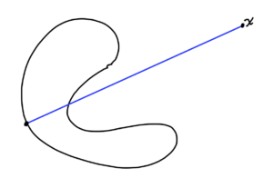
Here \( C \subseteq \mathbb{R}^n \) is not necessarily convex. We are using \( \sup \) here because the set \( C \) may be open. This function is the length of the line from \( \Bx \) to the point in \( C \) that is furthest from \( \Bx \).

  • \( \Bx – \By \) is linear in \( \Bx \)
  • \( g_\By(\Bx) = \Norm{\Bx – \By} \) is convex in \( \Bx \) since norms are convex functions.
  • \( F(\Bx) = \sup_{\By \in C} \Norm{ \Bx – \By } \). Each \( \By \) index is a convex function. Taking max of those.

Example:

\begin{equation}\label{eqn:convexOptimizationLecture7:600}
F(\Bx) = \inf_{\By \in C} \Norm{ \Bx – \By }.
\end{equation}

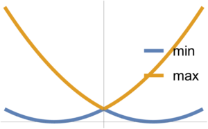
Min and max of two convex functions are plotted in fig. 4.

fig. 4. Min and max

The max is observed to be convex, whereas the min is not necessarily so.

\begin{equation}\label{eqn:convexOptimizationLecture7:800}
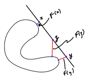
F(\Bz) = F(\theta \Bx + (1-\theta) \By) \ge \theta F(\Bx) + (1-\theta)F(\By).
\end{equation}

This is not necessarily convex for all sets \( C \subseteq \mathbb{R}^n \), because the \( \inf \) of a bunch of convex function is not necessarily convex. However, if \( C \) is convex, then \( F(\Bx) \) is convex.

Consequences of convexity for differentiable functions

  • Think about unconstrained functions \( \textrm{dom} F = \mathbb{R}^n \).
  • By first order condition \( F \) is convex iff the domain is convex and
    \begin{equation}\label{eqn:convexOptimizationLecture7:620}
    F(\Bx) \ge \lr{ \spacegrad F(\Bx)}^\T (\By – \Bx) \, \forall \Bx, \By \in \textrm{dom} F.
    \end{equation}

If \( F \) is convex and one can find an \( \Bx^\conj \in \textrm{dom} F \) such that

\begin{equation}\label{eqn:convexOptimizationLecture7:640}
\spacegrad F(\Bx^\conj) = 0,
\end{equation}

then

\begin{equation}\label{eqn:convexOptimizationLecture7:660}
F(\By) \ge F(\Bx^\conj) \, \forall \By \in \textrm{dom} F.
\end{equation}

If you can find the point where the gradient is zero (which can’t always be found), then \( \Bx^\conj\) is a global minimum of \( F \).

Conversely, if \( \Bx^\conj \) is a global minimizer of \( F \), then \( \spacegrad F(\Bx^\conj) = 0 \) must hold. If that were not the case, then you would be able to find a direction to move downhill, contracting the optimality of \( \Bx^\conj\).

Local vs Global optimum


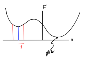
fig. 6. Global and local minimums

Definition: Local optimum
\( \Bx^\conj \) is a local optimum of \( F \) if \( \exists \epsilon > 0 \) such that \( \forall \Bx \), \( \Norm{\Bx – \Bx^\conj} < \epsilon \), we have

\begin{equation*}
F(\Bx^\conj) \le F(\Bx)
\end{equation*}


fig. 5. min length function

Theorem:
Suppose \( F \) is twice continuously differentiable (not necessarily convex)

  • If \( \Bx^\conj\) is a local optimum then\begin{equation*}
    \begin{aligned}
    \spacegrad F(\Bx^\conj) &= 0 \\
    \spacegrad^2 F(\Bx^\conj) \ge 0
    \end{aligned}
    \end{equation*}
  • If
    \begin{equation*}
    \begin{aligned}
    \spacegrad F(\Bx^\conj) &= 0 \\
    \spacegrad^2 F(\Bx^\conj) \ge 0
    \end{aligned},
    \end{equation*}then \( \Bx^\conj\) is a local optimum.

Proof:

  • Let \( \Bx^\conj \) be a local optimum. Pick any \( \Bv \in \mathbb{R}^n \).\begin{equation}\label{eqn:convexOptimizationLecture7:720}
    \lim_{t \rightarrow 0} \frac{ F(\Bx^\conj + t \Bv) – F(\Bx^\conj)}{t}
    = \lr{ \spacegrad F(\Bx^\conj) }^\T \Bv
    \ge 0.
    \end{equation}

Here the fraction is \( \ge 0 \) since \( \Bx^\conj \) is a local optimum.

Since the choice of \( \Bv \) is arbitrary, the only case that you can ensure that \( \ge 0, \forall \Bv \) is

\begin{equation}\label{eqn:convexOptimizationLecture7:740}
\spacegrad F = 0,
\end{equation}

( or else could pick \( \Bv = -\spacegrad F(\Bx^\conj) \).

This means that \( \spacegrad F(\Bx^\conj) = 0 \) if \( \Bx^\conj \) is a local optimum.

Consider the 2nd order derivative

\begin{equation}\label{eqn:convexOptimizationLecture7:760}
\begin{aligned}
\lim_{t \rightarrow 0} \frac{ F(\Bx^\conj + t \Bv) – F(\Bx^\conj)}{t^2}
&=
\lim_{t \rightarrow 0} \inv{t^2}
\lr{
F(\Bx^\conj) + t \lr{ \spacegrad F(\Bx^\conj) }^\T \Bv + \inv{2} t^2 \Bv^\T \spacegrad^2 F(\Bx^\conj) \Bv + O(t^3)
– F(\Bx^\conj)
} \\
&=
\inv{2} \Bv^\T \spacegrad^2 F(\Bx^\conj) \Bv \\
&\ge 0.
\end{aligned}
\end{equation}

Here the \( \ge \) condition also comes from the fraction, based on the optimiality of \( \Bx^\conj \). This is true for all choice of \( \Bv \), thus \( \spacegrad^2 F(\Bx^\conj) \).

References

[1] Stephen Boyd and Lieven Vandenberghe. Convex optimization. Cambridge university press, 2004.
ECE1505H Convex Optimization. Lecture 6: First and second order conditions. Taught by Prof.\ Stark Draper

February 1, 2017 ece1505 , , , , , , , ,

[Click here for a PDF of this post with nicer formatting]

Disclaimer

Peeter’s lecture notes from class. These may be incoherent and rough.

These are notes for the UofT course ECE1505H, Convex Optimization, taught by Prof. Stark Draper, from [1].

Today

  • First and second order conditions for convexity of differentiable functions.
  • Consequences of convexity: local and global optimality.
  • Properties.

Quasi-convex

\( F_1 \) and \( F_2 \) convex implies \( \max( F_1, F_2) \) convex.


fig. 1. Min and Max

Note that \( \min(F_1, F_2) \) is NOT convex.

If \( F : \mathbb{R}^n \rightarrow \mathbb{R} \) is convex, then \( F( \Bx_0 + t \Bv ) \) is convex in \( t\,\forall t \in \mathbb{R}, \Bx_0 \in \mathbb{R}^n, \Bv \in \mathbb{R}^n \), provided \( \Bx_0 + t \Bv \in \textrm{dom} F \).

Idea: Restrict to a line (line segment) in \( \textrm{dom} F \). Take a cross section or slice through \( F \) alone the line. If the result is a 1D convex function for all slices, then \( F \) is convex.

This is nice since it allows for checking for convexity, and is also nice numerically. Attempting to test a given data set for non-convexity with some random lines can help disprove convexity. However, to show that \( F \) is convex it is required to test all possible slices (which isn’t possible numerically, but is in some circumstances possible analytically).

Differentiable (convex) functions

Definition: First order condition.

If

\begin{equation*}
F : \mathbb{R}^n \rightarrow \mathbb{R}
\end{equation*}

is differentiable, then \( F \) is convex iff \( \textrm{dom} F \) is a convex set and \( \forall \Bx, \Bx_0 \in \textrm{dom} F \)

\begin{equation*}
F(\Bx) \ge F(\Bx_0) + \lr{\spacegrad F(\Bx_0)}^\T (\Bx – \Bx_0).
\end{equation*}

This is the first order Taylor expansion. If \( n = 1 \), this is \( F(x) \ge F(x_0) + F'(x_0) ( x – x_0) \).

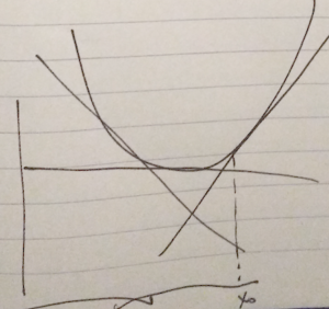
The first order condition says a convex function \underline{always} lies above its first order approximation, as sketched in fig. 3.


fig. 2. First order approximation lies below convex function

When differentiable, the supporting plane is the tangent plane.

Definition: Second order condition

If \( F : \mathbb{R}^n \rightarrow \mathbb{R} \) is twice differentiable, then \( F \) is convex iff \( \textrm{dom} F \) is a convex set and \( \spacegrad^2 F(\Bx) \ge 0 \,\forall \Bx \in \textrm{dom} F\).

The Hessian is always symmetric, but is not necessarily positive. Recall that the Hessian is the matrix of the second order partials \( (\spacegrad F)_{ij} = \partial^2 F/(\partial x_i \partial x_j) \).

The scalar case is \( F”(x) \ge 0 \, \forall x \in \textrm{dom} F \).

An implication is that if \( F \) is convex, then \( F(x) \ge F(x_0) + F'(x_0) (x – x_0) \,\forall x, x_0 \in \textrm{dom} F\)

Since \( F \) is convex, \( \textrm{dom} F \) is convex.

Consider any 2 points \( x, y \in \textrm{dom} F \), and \( \theta \in [0,1] \). Define

\begin{equation}\label{eqn:convexOptimizationLecture6:60}
z = (1-\theta) x + \theta y \in \textrm{dom} F,
\end{equation}

then since \( \textrm{dom} F \) is convex

\begin{equation}\label{eqn:convexOptimizationLecture6:80}
F(z) =
F( (1-\theta) x + \theta y )
\le
(1-\theta) F(x) + \theta F(y )
\end{equation}

Reordering

\begin{equation}\label{eqn:convexOptimizationLecture6:220}
\theta F(x) \ge
\theta F(x) + F(z) – F(x),
\end{equation}

or
\begin{equation}\label{eqn:convexOptimizationLecture6:100}
F(y) \ge
F(x) + \frac{F(x + \theta(y-x)) – F(x)}{\theta},
\end{equation}

which is, in the limit,

\begin{equation}\label{eqn:convexOptimizationLecture6:120}
F(y) \ge
F(x) + F'(x) (y – x),
\end{equation}

completing one direction of the proof.

To prove the other direction, showing that

\begin{equation}\label{eqn:convexOptimizationLecture6:140}
F(x) \ge F(x_0) + F'(x_0) (x – x_0),
\end{equation}

implies that \( F \) is convex. Take any \( x, y \in \textrm{dom} F \) and any \( \theta \in [0,1] \). Define

\begin{equation}\label{eqn:convexOptimizationLecture6:160}
z = \theta x + (1 -\theta) y,
\end{equation}

which is in \( \textrm{dom} F \) by assumption. We want to show that

\begin{equation}\label{eqn:convexOptimizationLecture6:180}
F(z) \le \theta F(x) + (1-\theta) F(y).
\end{equation}

By assumption

  1. \( F(x) \ge F(z) + F'(z) (x – z) \)
  2. \( F(y) \ge F(z) + F'(z) (y – z) \)

Compute

\begin{equation}\label{eqn:convexOptimizationLecture6:200}
\begin{aligned}
\theta F(x) + (1-\theta) F(y)
&\ge
\theta \lr{ F(z) + F'(z) (x – z) }
+ (1-\theta) \lr{ F(z) + F'(z) (y – z) } \\
&=
F(z) + F'(z) \lr{ \theta( x – z) + (1-\theta) (y-z) } \\
&=
F(z) + F'(z) \lr{ \theta x + (1-\theta) y – \theta z – (1 -\theta) z } \\
&=
F(z) + F'(z) \lr{ \theta x + (1-\theta) y – z} \\
&=
F(z) + F'(z) \lr{ z – z} \\
&= F(z).
\end{aligned}
\end{equation}

Proof of the 2nd order case for \( n = 1 \)

Want to prove that if

\begin{equation}\label{eqn:convexOptimizationLecture6:240}
F : \mathbb{R} \rightarrow \mathbb{R}
\end{equation}

is a convex function, then \( F”(x) \ge 0 \,\forall x \in \textrm{dom} F \).

By the first order conditions \( \forall x \ne y \in \textrm{dom} F \)

\begin{equation}\label{eqn:convexOptimizationLecture6:260}
\begin{aligned}
F(y) &\ge F(x) + F'(x) (y – x)
F(x) &\ge F(y) + F'(y) (x – y)
\end{aligned}
\end{equation}

Can combine and get

\begin{equation}\label{eqn:convexOptimizationLecture6:280}
F'(x) (y-x) \le F(y) – F(x) \le F'(y)(y-x)
\end{equation}

Subtract the two derivative terms for

\begin{equation}\label{eqn:convexOptimizationLecture6:340}
\frac{(F'(y) – F'(x))(y – x)}{(y – x)^2} \ge 0,
\end{equation}

or
\begin{equation}\label{eqn:convexOptimizationLecture6:300}
\frac{F'(y) – F'(x)}{y – x} \ge 0.
\end{equation}

In the limit as \( y \rightarrow x \), this is
\begin{equation}\label{eqn:convexOptimizationLecture6:320}
\boxed{
F”(x) \ge 0 \,\forall x \in \textrm{dom} F.
}
\end{equation}

Now prove the reverse condition:

If \( F”(x) \ge 0 \,\forall x \in \textrm{dom} F \subseteq \mathbb{R} \), implies that \( F : \mathbb{R} \rightarrow \mathbb{R} \) is convex.

Note that if \( F”(x) \ge 0 \), then \( F'(x) \) is non-decreasing in \( x \).

i.e. If \( x < y \), where \( x, y \in \textrm{dom} F\), then

\begin{equation}\label{eqn:convexOptimizationLecture6:360}
F'(x) \le F'(y).
\end{equation}

Consider any \( x,y \in \textrm{dom} F\) such that \( x < y \), where

\begin{equation}\label{eqn:convexOptimizationLecture6:380}
F(y) – F(x) = \int_x^y F'(t) dt \ge F'(x) \int_x^y 1 dt = F'(x) (y-x).
\end{equation}

This tells us that

\begin{equation}\label{eqn:convexOptimizationLecture6:400}
F(y) \ge F(x) + F'(x)(y – x),
\end{equation}

which is the first order condition. Similarly consider any \( x,y \in \textrm{dom} F\) such that \( x < y \), where

\begin{equation}\label{eqn:convexOptimizationLecture6:420}
F(y) – F(x) = \int_x^y F'(t) dt \le F'(y) \int_x^y 1 dt = F'(y) (y-x).
\end{equation}

This tells us that

\begin{equation}\label{eqn:convexOptimizationLecture6:440}
F(x) \ge F(y) + F'(y)(x – y).
\end{equation}

Vector proof:

\( F \) is convex iff \( F(\Bx + t \Bv) \) is convex \( \forall \Bx,\Bv \in \mathbb{R}^n, t \in \mathbb{R} \), keeping \( \Bx + t \Bv \in \textrm{dom} F\).

Let
\begin{equation}\label{eqn:convexOptimizationLecture6:460}
h(t ; \Bx, \Bv) = F(\Bx + t \Bv)
\end{equation}

then \( h(t) \) satisfies scalar first and second order conditions for all \( \Bx, \Bv \).

\begin{equation}\label{eqn:convexOptimizationLecture6:480}
h(t) = F(\Bx + t \Bv) = F(g(t)),
\end{equation}

where \( g(t) = \Bx + t \Bv \), where

\begin{equation}\label{eqn:convexOptimizationLecture6:500}
\begin{aligned}
F &: \mathbb{R}^n \rightarrow \mathbb{R} \\
g &: \mathbb{R} \rightarrow \mathbb{R}^n.
\end{aligned}
\end{equation}

This is expressing \( h(t) \) as a composition of two functions. By the first order condition for scalar functions we know that

\begin{equation}\label{eqn:convexOptimizationLecture6:520}
h(t) \ge h(0) + h'(0) t.
\end{equation}

Note that

\begin{equation}\label{eqn:convexOptimizationLecture6:540}
h(0) = \evalbar{F(\Bx + t \Bv)}{t = 0} = F(\Bx).
\end{equation}

Let’s figure out what \( h'(0) \) is. Recall hat for any \( \tilde{F} : \mathbb{R}^n \rightarrow \mathbb{R}^m \)

\begin{equation}\label{eqn:convexOptimizationLecture6:560}
D \tilde{F} \in \mathbb{R}^{m \times n},
\end{equation}

and
\begin{equation}\label{eqn:convexOptimizationLecture6:580}
{D \tilde{F}(\Bx)}_{ij} = \PD{x_j}{\tilde{F_i}(\Bx)}
\end{equation}

This is one function per row, for \( i \in [1,m], j \in [1,n] \). This gives

\begin{equation}\label{eqn:convexOptimizationLecture6:600}
\begin{aligned}
\frac{d}{dt} F(\Bx + \Bv t)
&=
\frac{d}{dt} F( g(t) ) \\
&=
\frac{d}{dt} h(t) \\
&= D h(t) \\
&= D F(g(t)) \cdot D g(t)
\end{aligned}
\end{equation}

The first matrix is in \( \mathbb{R}^{1\times n} \) whereas the second is in \( \mathbb{R}^{n\times 1} \), since \( F : \mathbb{R}^n \rightarrow \mathbb{R} \) and \( g : \mathbb{R} \rightarrow \mathbb{R}^n \). This gives

\begin{equation}\label{eqn:convexOptimizationLecture6:620}
\frac{d}{dt} F(\Bx + \Bv t)
= \evalbar{D F(\tilde{\Bx})}{\tilde{\Bx} = g(t)} \cdot D g(t).
\end{equation}

That first matrix is

\begin{equation}\label{eqn:convexOptimizationLecture6:640}
\begin{aligned}
\evalbar{D F(\tilde{\Bx})}{\tilde{\Bx} = g(t)}
&=
\evalbar{
\lr{\begin{bmatrix}
\PD{\tilde{x}_1}{ F(\tilde{\Bx})} &
\PD{\tilde{x}_2}{ F(\tilde{\Bx})} & \cdots
\PD{\tilde{x}_n}{ F(\tilde{\Bx})}
\end{bmatrix}
}}{ \tilde{\Bx} = g(t) = \Bx + t \Bv } \\
&=
\evalbar{
\lr{ \spacegrad F(\tilde{\Bx}) }^\T
}{
\tilde{\Bx} = g(t)
} \\
=
\lr{ \spacegrad F(g(t)) }^\T.
\end{aligned}
\end{equation}

The second Jacobian is

\begin{equation}\label{eqn:convexOptimizationLecture6:660}
D g(t)
=
D
\begin{bmatrix}
g_1(t) \\
g_2(t) \\
\vdots \\
g_n(t) \\
\end{bmatrix}
=
D
\begin{bmatrix}
x_1 + t v_1 \\
x_2 + t v_2 \\
\vdots \\
x_n + t v_n \\
\end{bmatrix}
=
\begin{bmatrix}
v_1 \\
v_1 \\
\vdots \\
v_n \\
\end{bmatrix}
=
\Bv.
\end{equation}

so

\begin{equation}\label{eqn:convexOptimizationLecture6:680}
h'(t) = D h(t) = \lr{ \spacegrad F(g(t))}^\T \Bv,
\end{equation}

and
\begin{equation}\label{eqn:convexOptimizationLecture6:700}
h'(0) = \lr{ \spacegrad F(g(0))}^\T \Bv
=
\lr{ \spacegrad F(\Bx)}^\T \Bv.
\end{equation}

Finally

\begin{equation}\label{eqn:convexOptimizationLecture6:720}
\begin{aligned}
F(\Bx + t \Bv)
&\ge h(0) + h'(0) t \\
&= F(\Bx) + \lr{ \spacegrad F(\Bx) }^\T (t \Bv) \\
&= F(\Bx) + \innerprod{ \spacegrad F(\Bx) }{ t \Bv}.
\end{aligned}
\end{equation}

Which is true for all \( \Bx, \Bx + t \Bv \in \textrm{dom} F \). Note that the quantity \( t \Bv \) is a shift.

Epigraph

Recall that if \( (\Bx, t) \in \textrm{epi} F \) then \( t \ge F(\Bx) \).

\begin{equation}\label{eqn:convexOptimizationLecture6:740}
t \ge F(\Bx) \ge F(\Bx_0) + \lr{\spacegrad F(\Bx_0) }^\T (\Bx – \Bx_0),
\end{equation}

or

\begin{equation}\label{eqn:convexOptimizationLecture6:760}
0 \ge
-(t – F(\Bx_0)) + \lr{\spacegrad F(\Bx_0) }^\T (\Bx – \Bx_0),
\end{equation}

In block matrix form

\begin{equation}\label{eqn:convexOptimizationLecture6:780}
0 \ge
\begin{bmatrix}
\lr{ \spacegrad F(\Bx_0) }^\T & -1
\end{bmatrix}
\begin{bmatrix}
\Bx – \Bx_0 \\
t – F(\Bx_0)
\end{bmatrix}
\end{equation}

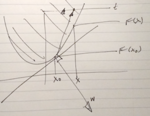
With \( \Bw =
\begin{bmatrix}
\lr{ \spacegrad F(\Bx_0) }^\T & -1
\end{bmatrix} \), the geometry of the epigraph relation to the half plane is sketched in fig. 3.


fig. 3. Half planes and epigraph.

References

[1] Stephen Boyd and Lieven Vandenberghe. Convex optimization. Cambridge university press, 2004.
ECE1505H Convex Optimization. Lecture 5: Sets, epigraphs, quasi-convexity, and sublevel sets. Taught by Prof. Stark Draper

January 26, 2017 ece1505 , , , , , , , ,

[Click here for a PDF of this post with nicer formatting]

Disclaimer

Peeter’s lecture notes from class. These may be incoherent and rough.

These are notes for the UofT course ECE1505H, Convex Optimization, taught by Prof. Stark Draper, from [1].

Last time

  • examples of sets: planes, half spaces, balls, ellipses, cone of positive semi-definite matrices
  • generalized inequalities
  • examples of convexity preserving operations

Today

  • more examples of convexity preserving operations
  • separating and supporting hyperplanes
  • basic definitions of convex functions
  • epigraphs, quasi-convexity, sublevel sets
  • first and second order conditions for convexity of differentiable functions.

Operations that preserve convexity

If \( S_\alpha \) is convex \( \forall \alpha \in A \), then

\begin{equation}\label{eqn:convexOptimizationLecture5:40}
\cup_{\alpha \in A} S_\alpha,
\end{equation}

is convex.

Example:

\begin{equation}\label{eqn:convexOptimizationLecture5:60}
F(\Bx) = A \Bx + \Bb
\end{equation}

\begin{equation}\label{eqn:convexOptimizationLecture5:80}
\begin{aligned}
\Bx &\in \mathbb{R}^n \\
A &\in \mathbb{R}^{m \times n} \\
F &: \mathbb{R}^{n} \rightarrow \mathbb{R}^m \\
\Bb &\in \mathbb{R}^m
\end{aligned}
\end{equation}

  1. If \( S \in \mathbb{R}^n \) is convex, then\begin{equation}\label{eqn:convexOptimizationLecture5:100}
    F(S) = \setlr{ F(\Bx) | \Bx \in S }
    \end{equation}is convex if \( F \) is affine.
  2. If \( S \in \mathbb{R}^m \) is convex, then\begin{equation}\label{eqn:convexOptimizationLecture5:120}
    F^{-1}(S) = \setlr{ \Bx | F(\Bx) \in S }
    \end{equation}

    is convex.

Example:

\begin{equation}\label{eqn:convexOptimizationLecture5:140}
\setlr{ \By | \By = A \Bx + \Bb, \Norm{\Bx} \le 1}
\end{equation}

is convex. Here \( A \Bx + \Bb \) is an affine function (\(F(\Bx)\). This is the image of a (convex) unit ball, through an affine map.

Earlier saw when defining ellipses

\begin{equation}\label{eqn:convexOptimizationLecture5:160}
\By = P^{1/2} \Bx + \Bx_c
\end{equation}

Example :

\begin{equation}\label{eqn:convexOptimizationLecture5:180}
\setlr{ \Bx | \Norm{ A \Bx + \Bb } \le 1 },
\end{equation}

is convex. This can be seen by writing

\begin{equation}\label{eqn:convexOptimizationLecture5:200}
\begin{aligned}
\setlr{ \Bx | \Norm{ A \Bx + \Bb } \le 1 }
&=
\setlr{ \Bx | \Norm{ F(\Bx) } \le 1 } \\
&=
\setlr{ \Bx | F(\Bx) \in \mathcal{B} },
\end{aligned}
\end{equation}

where \( \mathcal{B} = \setlr{ \By | \Norm{\By} \le 1 } \). This is the pre-image (under \(F()\)) of a unit norm ball.

Example:

\begin{equation}\label{eqn:convexOptimizationLecture5:220}
\setlr{ \Bx \in \mathbb{R}^n | x_1 A_1 + x_2 A_2 + \cdots x_n A_n \le \mathcal{B} }
\end{equation}

where \( A_i \in S^m \) and \( \mathcal{B} \in S^m \), and the inequality is a matrix inequality. This is a convex set. The constraint is a “linear matrix inequality” (LMI).

This has to do with an affine map:

\begin{equation}\label{eqn:convexOptimizationLecture5:240}
F(\Bx) = B – 1 x_1 A_1 – x_2 A_2 – \cdots x_n A_n \ge 0
\end{equation}

(positive semi-definite inequality). This is a mapping

\begin{equation}\label{eqn:convexOptimizationLecture5:480}
F : \mathbb{R}^n \rightarrow S^m,
\end{equation}

since all \( A_i \) and \( B \) are in \( S^m \).

This \( F(\Bx) = B – A(\Bx) \) is a constant and a factor linear in x, so is affine. Can be written

\begin{equation}\label{eqn:convexOptimizationLecture5:260}
\setlr{ \Bx | B – A(\Bx) \ge 0 }
=
\setlr{ \Bx | B – A(\Bx) \in S^m_{+} }
\end{equation}

This is a pre-image of a cone of PSD matrices, which is convex. Therefore, this is a convex set.

Separating hyperplanes

Theorem: Separating hyperplanes

If \( S, T \subseteq \mathbb{R}^n \) are convex and disjoint
i.e. \( S \cup T = 0\), then
there exists on \( \Ba \in \mathbb{R}^n \) \( \Ba \ne 0 \) and a \( \Bb \in \mathbb{R}^n \) such that

\begin{equation*}
\Ba^\T \Bx \ge \Bb \, \forall \Bx \in S
\end{equation*}

and
\begin{equation*}
\Ba^\T \Bx < \Bb \,\forall \Bx \in T.
\end{equation*}

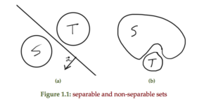
An example of a hyperplanes that separates two sets and two sets that are not separable is sketched in fig 1.1

Proof in the book.

Theorem: Supporting hyperplane
If \( S \) is convex then \( \forall x_0 \in \partial S = \textrm{cl}(S) \ \textrm{int}(S) \), where
\( \partial S \) is the boundary of \( S \), then \( \exists \) an \( \Ba \ne 0 \in \mathbb{R}^n \) such that \( \Ba^\T \Bx \le \Ba^\T x_0 \, \forall \Bx \in S \).

Here \( \ \) denotes “without”.

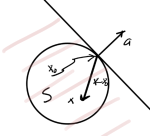
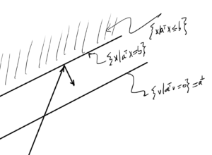
An example is sketched in fig. 3, for which

fig. 3. Supporting hyperplane.

  • The vector \( \Ba \) perpendicular to tangent plane.
  • inner product \( \Ba^\T (\Bx – \Bx_0) \le 0 \).

A set with a supporting hyperplane is sketched in fig 4a whereas fig 4b shows that there is not necessarily a unique supporting hyperplane at any given point, even if \( S \) is convex.


fig 4a. Set with supporting hyperplane.


fig 4b. No unique supporting hyperplane possible.

basic definitions of convex functions

Theorem: Convex functions
If \( F : \mathbb{R}^n \rightarrow \mathbb{R} \) is defined on a convex domain (i.e. \( \textrm{dom} F \subseteq \mathbb{R}^n \) is a convex set), then \( F \) is convex if \( \forall \Bx, \By \in \textrm{dom} F \), \( \forall \theta \in [0,1] \in \mathbb{R} \)

\begin{equation}\label{eqn:convexOptimizationLecture5:340}
F( \theta \Bx + (1-\theta) \By \le \theta F(\Bx) + (1-\theta) F(\By)
\end{equation}

An example is sketched in fig. 5.


fig. 5. Example of convex function.

Remarks

  • Require \( \textrm{dom} F \) to be a convex set. This is required so that the function at the point \( \theta u + (1-\theta) v \) can be evaluated. i.e. so that \( F(\theta u + (1-\theta) v) \) is well defined. Example: \( \textrm{dom} F = (-\infty, 0] \cup [1, \infty) \) is not okay, because a linear combination in \( (0,1) \) would be undesirable.
  • Parameter \( \theta \) is “how much up” the line segment connecting \( (u, F(u) \) and \( (v, F(v) \). This line segment never below the bottom of the bowl.
    The function is \underlineAndIndex{concave}, if \( -F \) is convex.
    i.e. If the convex function is flipped upside down. That is\begin{equation}\label{eqn:convexOptimizationLecture5:360}
    F(\theta \Bx + (1-\theta) \By ) \ge \theta F(\Bx) + (1-\theta) F(\By) \,\forall \Bx,\By \in \textrm{dom} F, \theta \in [0,1].
    \end{equation}
  • a “strictly” convex function means \(\forall \theta \in [0,1] \)\begin{equation}\label{eqn:convexOptimizationLecture5:380}
    F(\theta \Bx + (1-\theta) \By ) < \theta F(\Bx) + (1-theta) F(\By).
    \end{equation}
  • Strictly concave function \( F \) means \( -F \) is strictly convex.
  • Examples:\imageFigure{../figures/ece1505-convex-optimization/l5Fig6a}{}{fig:l5:l5Fig6a}{0.2}

    fig 6a. Not convex or concave.


    fig 6b. Not strictly convex

Definition: Epigraph of a function

The epigraph \( \textrm{epi} F \) of a function \( F : \mathbb{R}^n \rightarrow \mathbb{R} \) is

\begin{equation*}
\textrm{epi} F = \setlr{ (\Bx,t) \in \mathbb{R}^{n +1} | \Bx \in \textrm{dom} F, t \ge F(\Bx) },
\end{equation*}

where \( \Bx \in \mathbb{R}^n, t \in \mathbb{R} \).


fig. 7. Epigraph.

Theorem: Convexity and epigraph.
If \( F \) is convex implies \( \textrm{epi} F \) is a convex set.

Proof:

For convex function, a line segment connecting any 2 points on function is above the function. i.e. it is \( \textrm{epi} F \).

Many authors will go the other way around, showing \ref{dfn:convexOptimizationLecture5:400} from \ref{thm:convexOptimizationLecture5:420}. That is:

Pick any 2 points in \( \textrm{epi} F \), \( (\Bx,\mu) \in \textrm{epi} F\) and \( (\By, \nu) \in \textrm{epi} F \). Consider convex combination

\begin{equation}\label{eqn:convexOptimizationLecture5:420}
\theta( \Bx, \mu ) + (1-\theta) (\By, \nu) =
(\theta \Bx (1-\theta) \By, \theta \mu (1-\theta) \nu )
\in \textrm{epi} F,
\end{equation}

since \( \textrm{epi} F \) is a convex set.

By definition of \( \textrm{epi} F \)

\begin{equation}\label{eqn:convexOptimizationLecture5:440}
F( \theta \Bx (1-\theta) \By ) \le \theta \mu (1-\theta) \nu.
\end{equation}

Picking \( \mu = F(\Bx), \nu = F(\By) \) gives
\begin{equation}\label{eqn:convexOptimizationLecture5:460}
F( \theta \Bx (1-\theta) \By ) \le \theta F(\Bx) (1-\theta) F(\By).
\end{equation}

Extended value function

Sometimes convenient to work with “extended value function”

\begin{equation}\label{eqn:convexOptimizationLecture5:500}
\tilde{F}(\Bx) =
\left\{
\begin{array}{l l}
F(\Bx) & \quad \mbox{If \( \Bx \in \textrm{dom} F\)} \\
\infty & \quad \mbox{otherwise.}
\end{array}
\right.
\end{equation}

Examples:

  • Linear (affine) functions (fig. 8) are both convex and concave.

    fig. 8. Linear functions.

  • \( x^2 \) is convex, sketched in fig. 9.

    fig. 9. Convex (quadratic.)

  • \( \log x, \textrm{dom} F = \mathbb{R}_{+} \) concave, sketched in fig. 10.

    fig. 10. Concave (logarithm.)

  • \( \Norm{\Bx} \) is convex. \( \Norm{ \theta \Bx + (1-\theta) \By } \le \theta \Norm{ \Bx } + (1-\theta) \Norm{\By } \).
  • \( 1/x \) is convex on \( \setlr{ x | x > 0 } = \textrm{dom} F \), and concave on \( \setlr{ x | x < 0 } = \textrm{dom} F \). \begin{equation}\label{eqn:convexOptimizationLecture5:520} \tilde{F}(x) = \left\{ \begin{array}{l l} \inv{x} & \quad \mbox{If \( x > 0 \)} \\
    \infty & \quad \mbox{else.}
    \end{array}
    \right.
    \end{equation}

Definition: Sublevel

The sublevel set of a function \( F : \mathbb{R}^n \rightarrow \mathbb{R} \) is

\begin{equation*}
C(\alpha) = \setlr{ \Bx \in \textrm{dom} F | F(\Bx) \le \alpha }
\end{equation*}


Convex sublevel


Non-convex sublevel.

Theorem:
If \( F \) is convex then \( C(\alpha) \) is a convex set \( \forall \alpha \).

This is not an if and only if condition, as illustrated in fig. 12.


fig. 12. Convex sublevel does not imply convexity.

There \( C(\alpha) \) is convex, but the function itself is not.

Proof:

Since \( F \) is convex, then \( \textrm{epi} F \) is a convex set.

  • Let\begin{equation}\label{eqn:convexOptimizationLecture5:580}
    \mathcal{A} = \setlr{ (\Bx,t) | t = \alpha }
    \end{equation}is a convex set.
  • \( \mathcal{A} \cap \textrm{epi} F \)is a convex set since it is the intersection of convex sets.
  • Project \( \mathcal{A} \cap \textrm{epi} F \) onto \R{n} (i.e. domain of \( F \) ). The projection is an affine mapping. Image of a convex set through affine mapping is a convex set.

Definition: Quasi-convex.

A function is quasi-convex if \underline{all} of its sublevel sets are convex.

Composing convex functions

Properties of convex functions:

  • If \( F \) is convex, then \( \alpha F \) is convex \( \forall \alpha > 0 \).
  • If \( F_1, F_2 \) are convex, then the sum \( F_1 + F_2 \) is convex.
  • If \( F \) is convex, then \( g(\Bx) = F(A \Bx + \Bb) \) is convex \( \forall \Bx \in \setlr{ \Bx | A \Bx + \Bb \in \textrm{dom} F } \).

Note: for the last

\begin{equation}\label{eqn:convexOptimizationLecture5:620}
\begin{aligned}
g &: \mathbb{R}^m \rightarrow \mathbb{R} \\
F &: \mathbb{R}^n \rightarrow \mathbb{R} \\
\Bx &\in \mathbb{R}^m \\
A &\in \mathbb{R}^{n \times m} \\
\Bb &\in \mathbb{R}^n
\end{aligned}
\end{equation}

Proof (of last):

\begin{equation}\label{eqn:convexOptimizationLecture5:640}
\begin{aligned}
g( \theta \Bx + (1-\theta) \By )
&=
F( \theta (A \Bx + \Bb) + (1-\theta) (A \By + \Bb) ) \\
&\le
\theta F( A \Bx + \Bb) + (1-\theta) F (A \By + \Bb) \\
&= \theta g(\Bx) + (1-\theta) g(\By).
\end{aligned}
\end{equation}

References

[1] Stephen Boyd and Lieven Vandenberghe. Convex optimization. Cambridge university press, 2004.
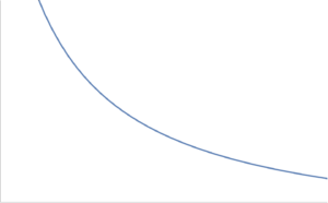
ECE1505H Convex Optimization. Lecture 4: Sets and convexity. Taught by Prof. Stark Draper

January 25, 2017 ece1505 , , , , , , ,

ECE1505H Convex Optimization. Lecture 4: Sets and convexity. Taught by Prof. Stark Draper

[Click here for a PDF of this post with nicer formatting]

Disclaimer

Peeter’s lecture notes from class. These may be incoherent and rough.

These are notes for the UofT course ECE1505H, Convex Optimization, taught by Prof. Stark Draper, covering [1] content.

Today

  • more on various sets: hyperplanes, half-spaces, polyhedra, balls, ellipses, norm balls, cone of PSD
  • generalize inequalities
  • operations that preserve convexity
  • separating and supporting hyperplanes.

Hyperplanes

Find some \( \Bx_0 \in \mathbb{R}^n \) such that \( \Ba^\T \Bx_0 = \Bb \), so

\begin{equation}\label{eqn:convexOptimizationLecture4:20}
\begin{aligned}
\setlr{ \Bx | \Ba^\T \Bx = \Bb }
&=
\setlr{ \Bx | \Ba^\T \Bx = \Ba^\T \Bx_0 } \\
&=
\setlr{ \Bx | \Ba^\T (\Bx – \Bx_0) } \\
&=
\Bx_0 + \Ba^\perp,
\end{aligned}
\end{equation}

where

\begin{equation}\label{eqn:convexOptimizationLecture4:40}
\Ba^\perp = \setlr{ \Bv | \Ba^\T \Bv = 0 }.
\end{equation}

fig. 1. Parallel hyperplanes.


Recall

\begin{equation}\label{eqn:convexOptimizationLecture4:60}
\Norm{\Bz}_\conj = \sup_\Bx \setlr{ \Bz^\T \Bx | \Norm{\Bx} \le 1 }
\end{equation}

Denote the optimizer of above as \( \Bx^\conj \). By definition

\begin{equation}\label{eqn:convexOptimizationLecture4:80}
\Bz^\T \Bx^\conj \ge \Bz^\T \Bx \quad \forall \Bx, \Norm{\Bx} \le 1
\end{equation}

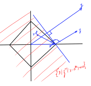
This defines a half space in which the unit ball

\begin{equation}\label{eqn:convexOptimizationLecture4:100}
\setlr{ \Bx | \Bz^\T (\Bx – \Bx^\conj \le 0 }
\end{equation}

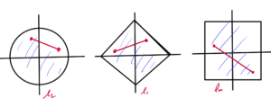
Start with the \( l_1 \) norm, duals of \( l_1 \) is \( l_\infty \)


fig. 2. Half space containing unit ball.

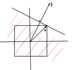
Similar pic for \( l_\infty \), for which the dual is the \( l_1 \) norm, as sketched in fig. 3.  Here the optimizer point is at \( (1,1) \)


fig. 3. Half space containing the unit ball for l_infinity

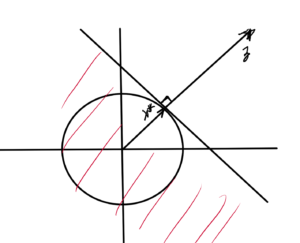
and a similar pic for \( l_2 \), which is sketched in fig. 4.
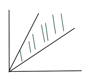
 

fig. 4. Half space containing for l_2 unit ball.
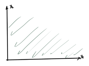
Q: What was this optimizer point?

Polyhedra

\begin{equation}\label{eqn:convexOptimizationLecture4:120}
\begin{aligned}
\mathcal{P}
&= \setlr{ \Bx |
\Ba_j^\T \Bx \le \Bb_j, j \in [1,m],
\Bc_i^\T \Bx = \Bd_i, i \in [1,p]
} \\
&=
\setlr{ \Bx | A \Bx \le \Bb, C \Bx = d },
\end{aligned}
\end{equation}

where the final inequality and equality are component wise.

Proving \( \mathcal{P} \) is convex:

  • Pick \(\Bx_1 \in \mathcal{P}\), \(\Bx_2 \in \mathcal{P} \)
  • Pick any \(\theta \in [0,1]\)
  • Test \( \theta \Bx_1 + (1-\theta) \Bx_2 \). Is it in \(\mathcal{P}\)?

\begin{equation}\label{eqn:convexOptimizationLecture4:140}
\begin{aligned}
A \lr{ \theta \Bx_1 + (1-\theta) \Bx_2 }
&=
\theta A \Bx_1 + (1-\theta) A \Bx_2 \\
&\le
\theta \Bb + (1-\theta) \Bb \\
&=
\Bb.
\end{aligned}
\end{equation}

Balls

Euclidean ball for \( \Bx_c \in \mathbb{R}^n, r \in \mathbb{R} \)

\begin{equation}\label{eqn:convexOptimizationLecture4:160}
\mathcal{B}(\Bx_c, r)
= \setlr{ \Bx | \Norm{\Bx – \Bx_c}_2 \le r },
\end{equation}

or
\begin{equation}\label{eqn:convexOptimizationLecture4:180}
\mathcal{B}(\Bx_c, r)
= \setlr{ \Bx | \lr{\Bx – \Bx_c}^\T \lr{\Bx – \Bx_c} \le r^2 }.
\end{equation}

Let \( \Bx_1, \Bx_2 \), \(\theta \in [0,1]\)

\begin{equation}\label{eqn:convexOptimizationLecture4:200}
\begin{aligned}
\Norm{ \theta \Bx_1 + (1-\theta) \Bx_2 – \Bx_c }_2
&=
\Norm{ \theta (\Bx_1 – \Bx_c) + (1-\theta) (\Bx_2 – \Bx_c) }_2 \\
&\le
\Norm{ \theta (\Bx_1 – \Bx_c)}_2 + \Norm{(1-\theta) (\Bx_2 – \Bx_c) }_2 \\
&=
\Abs{\theta} \Norm{ \Bx_1 – \Bx_c}_2 + \Abs{1 -\theta} \Norm{ \Bx_2 – \Bx_c }_2 \\
&=
\theta \Norm{ \Bx_1 – \Bx_c}_2 + \lr{1 -\theta} \Norm{ \Bx_2 – \Bx_c }_2 \\
&\le
\theta r + (1 – \theta) r \\
&= r
\end{aligned}
\end{equation}

Ellipse

\begin{equation}\label{eqn:convexOptimizationLecture4:220}
\mathcal{E}(\Bx_c, P)
=
\setlr{ \Bx | (\Bx – \Bx_c)^\T P^{-1} (\Bx – \Bx_c) \le 1 },
\end{equation}

where \( P \in S^n_{++} \).

  • Euclidean ball is an ellipse with \( P = I r^2 \)
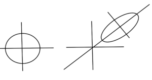
  • Ellipse is image of Euclidean ball \( \mathcal{B}(0,1) \) under affine mapping.


fig. 5. Circle and ellipse.

Given

\begin{equation}\label{eqn:convexOptimizationLecture4:240}
F(\Bu) = P^{1/2} \Bu + \Bx_c
\end{equation}

\begin{equation}\label{eqn:convexOptimizationLecture4:260}
\begin{aligned}
\setlr{ F(\Bu) | \Norm{\Bu}_2 \le r }
&=
\setlr{ P^{1/2} \Bu + \Bx_c | \Bu^\T \Bu \le r^2 } \\
&=
\setlr{ \Bx | \Bx = P^{1/2} \Bu + \Bx_c, \Bu^\T \Bu \le r^2 } \\
&=
\setlr{ \Bx | \Bu = P^{-1/2} (\Bx – \Bx_c), \Bu^\T \Bu \le r^2 } \\
&=
\setlr{ \Bx | (\Bx – \Bx_c)^\T P^{-1} (\Bx – \Bx_c) \le r^2 }
\end{aligned}
\end{equation}

Geometry of an ellipse

Decomposition of positive definite matrix \( P \in S^n_{++} \subset S^n \) is:

\begin{equation}\label{eqn:convexOptimizationLecture4:280}
\begin{aligned}
P &= Q \textrm{diag}(\lambda_i) Q^\T \\
Q^\T Q &= 1
\end{aligned},
\end{equation}

where \( \lambda_i \in \mathbb{R}\), and \(\lambda_i > 0 \). The ellipse is defined by

\begin{equation}\label{eqn:convexOptimizationLecture4:300}
(\Bx – \Bx_c)^\T Q \textrm{diag}(1/\lambda_i) (\Bx – \Bx_c) Q \le r^2
\end{equation}

The term \( (\Bx – \Bx_c)^\T Q \) projects \( \Bx – \Bx_c \) onto the columns of \( Q \). Those columns are perpendicular since \( Q \) is an orthogonal matrix. Let

\begin{equation}\label{eqn:convexOptimizationLecture4:320}
\tilde{\Bx} = Q^\T (\Bx – \Bx_c),
\end{equation}

this shifts the origin around \( \Bx_c \) and \( Q \) rotates into a new coordinate system. The ellipse is therefore

\begin{equation}\label{eqn:convexOptimizationLecture4:340}
\tilde{\Bx}^\T
\begin{bmatrix}
\inv{\lambda_1} & & & \\
&\inv{\lambda_2} & & \\
& \ddots & \\
& & & \inv{\lambda_n}
\end{bmatrix}
\tilde{\Bx}
=
\sum_{i = 1}^n \frac{\tilde{x}_i^2}{\lambda_i} \le 1.
\end{equation}

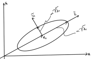
An example is sketched for \( \lambda_1 > \lambda_2 \) below.


Ellipse with \( \lambda_1 > \lambda_2 \).

  • \( \lambda_i \) tells us length of the semi-major axis.
  • Larger \( \lambda_i \) means \( \tilde{x}_i^2 \) can be bigger and still satisfy constraint \( \le 1 \).
  • Volume of ellipse if proportional to \( \sqrt{ \det P } = \sqrt{ \prod_{i = 1}^n \lambda_i } \).
  • When any \( \lambda_i \rightarrow 0 \) a dimension is lost and the volume goes to zero. That removes the invertibility required.

Ellipses will be seen a lot in this course, since we are interested in “bowl” like geometries (and the ellipse is the image of a Euclidean ball).

Norm ball.

The norm ball

\begin{equation}\label{eqn:convexOptimizationLecture4:360}
\mathcal{B} = \setlr{ \Bx | \Norm{\Bx} \le 1 },
\end{equation}

is a convex set for all norms. Proof:

Take any \( \Bx, \By \in \mathcal{B} \)

\begin{equation}\label{eqn:convexOptimizationLecture4:380}
\Norm{ \theta \Bx + (1 – \theta) \By }
\le
\Abs{\theta} \Norm{ \Bx } + \Abs{1 – \theta} \Norm{ \By }
=
\theta \Norm{ \Bx } + \lr{1 – \theta} \Norm{ \By }
\lr
\theta + \lr{1 – \theta}
=
1.
\end{equation}

This is true for any p-norm \( 1 \le p \), \( \Norm{\Bx}_p = \lr{ \sum_{i = 1}^n \Abs{x_i}^p }^{1/p} \).


Norm ball.

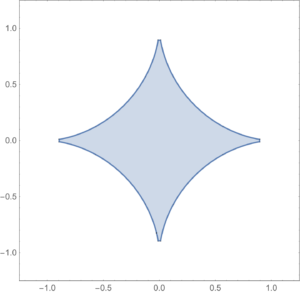
The shape of a \( p < 1 \) norm unit ball is sketched below (lines connecting points in such a region can exit the region).


Cones

Recall that \( C \) is a cone if \( \forall \Bx \in C, \theta \ge 0, \theta \Bx \in C \).

Impt cone of PSD matrices

\begin{equation}\label{eqn:convexOptimizationLecture4:400}
\begin{aligned}
S^n &= \setlr{ X \in \mathbb{R}^{n \times n} | X = X^\T } \\
S^n_{+} &= \setlr{ X \in S^n | \Bv^\T X \Bv \ge 0, \quad \forall v \in \mathbb{R}^n } \\
S^n_{++} &= \setlr{ X \in S^n_{+} | \Bv^\T X \Bv > 0, \quad \forall v \in \mathbb{R}^n } \\
\end{aligned}
\end{equation}

These have respectively

  • \( \lambda_i \in \mathbb{R} \)
  • \( \lambda_i \in \mathbb{R}_{+} \)
  • \( \lambda_i \in \mathbb{R}_{++} \)

\( S^n_{+} \) is a cone if:

\( X \in S^n_{+}\), then \( \theta X \in S^n_{+}, \quad \forall \theta \ge 0 \)

\begin{equation}\label{eqn:convexOptimizationLecture4:420}
\Bv^\T (\theta X) \Bv
= \theta \Bv^\T \Bv
\ge 0,
\end{equation}

since \( \theta \ge 0 \) and because \( X \in S^n_{+} \).

Shorthand:

\begin{equation}\label{eqn:convexOptimizationLecture4:440}
\begin{aligned}
X &\in S^n_{+} \Rightarrow X \succeq 0
X &\in S^n_{++} \Rightarrow X \succ 0.
\end{aligned}
\end{equation}

Further \( S^n_{+} \) is a convex cone.

Let \( A \in S^n_{+} \), \( B \in S^n_{+} \), \( \theta_1, \theta_2 \ge 0, \theta_1 + \theta_2 = 1 \), or \( \theta_2 = 1 – \theta_1 \).

Show that \( \theta_1 A + \theta_2 B \in S^n_{+} \) :

\begin{equation}\label{eqn:convexOptimizationLecture4:460}
\Bv^\T \lr{ \theta_1 A + \theta_2 B } \Bv
=
\theta_1 \Bv^\T A \Bv
+\theta_2 \Bv^\T B \Bv
\ge 0,
\end{equation}

since \( \theta_1 \ge 0, \theta_2 \ge 0, \Bv^\T A \Bv \ge 0, \Bv^\T B \Bv \ge 0 \).


fig. 8. Cone.

Inequalities:

Start with a proper cone \( K \subseteq \mathbb{R}^n \)

  • closed, convex
  • non-empty interior (“solid”)
  • “pointed” (contains no lines)

The \( K \) defines a generalized inequality in \R{n} defined as “\(\le_K\)”

Interpreting

\begin{equation}\label{eqn:convexOptimizationLecture4:480}
\begin{aligned}
\Bx \le_K \By &\leftrightarrow \By – \Bx \in K
\Bx \end{aligned}
\end{equation}

Why pointed? Want if \( \Bx \le_K \By \) and \( \By \le_K \Bx \) with this \( K \) is a half space.

Example:1: \( K = \mathbb{R}^n_{+}, \Bx \in \mathbb{R}^n, \By \in \mathbb{R}^n \)


fig. 12. K is non-negative “orthant”

\begin{equation}\label{eqn:convexOptimizationLecture4:500}
\Bx \le_K \By \Rightarrow \By – \Bx \in K
\end{equation}

say:

\begin{equation}\label{eqn:convexOptimizationLecture4:520}
\begin{bmatrix}
y_1 – x_1
y_2 – x_2
\end{bmatrix}
\in R^2_{+}
\end{equation}

Also:

\begin{equation}\label{eqn:convexOptimizationLecture4:540}
K = R^1_{+}
\end{equation}

(pointed, since it contains no rays)

\begin{equation}\label{eqn:convexOptimizationLecture4:560}
\Bx \le_K \By ,
\end{equation}

with respect to \( K = \mathbb{R}^n_{+} \) means that \( x_i \le y_i \) for all \( i \in [1,n]\).

Example:2: For \( K = PSD \subseteq S^n \),

\begin{equation}\label{eqn:convexOptimizationLecture4:580}
\Bx \le_K \By ,
\end{equation}

means that

\begin{equation}\label{eqn:convexOptimizationLecture4:600}
\By – \Bx \in K = S^n_{+}.
\end{equation}

  • Difference \( \By – \Bx \) is always in \( S \)
  • check if in \( K \) by checking if all eigenvalues \( \ge 0 \).
  • \( S^n_{++} \) is the interior of \( S^n_{+} \).

Interpretation:

\begin{equation}\label{eqn:convexOptimizationLecture4:620}
\begin{aligned}
\Bx \le_K \By &\leftrightarrow \By – \Bx \in K \\
\Bx \end{aligned}
\end{equation}

We’ll use these with vectors and matrices so often the \( K \) subscript will often be dropped, writing instead (for vectors)

\begin{equation}\label{eqn:convexOptimizationLecture4:640}
\begin{aligned}
\Bx \le \By &\leftrightarrow \By – \Bx \in \mathbb{R}^n_{+} \\
\Bx < \By &\leftrightarrow \By – \Bx \in \textrm{int} \mathbb{R}^n_{++}
\end{aligned}
\end{equation}

and for matrices

\begin{equation}\label{eqn:convexOptimizationLecture4:660}
\begin{aligned}
\Bx \le \By &\leftrightarrow \By – \Bx \in S^n_{+} \\
\Bx < \By &\leftrightarrow \By – \Bx \in \textrm{int} S^n_{++}.
\end{aligned}
\end{equation}

Intersection

Take the intersection of (perhaps infinitely many) sets \( S_\alpha \):

If \( S_\alpha \) is (affine,convex, conic) for all \( \alpha \in A \) then

\begin{equation}\label{eqn:convexOptimizationLecture4:680}
\cap_\alpha S_\alpha
\end{equation}

is (affine,convex, conic). To prove in homework:

\begin{equation}\label{eqn:convexOptimizationLecture4:700}
\mathcal{P} = \setlr{ \Bx | \Ba_i^\T \Bx \le \Bb_i, \Bc_j^\T \Bx = \Bd_j, \quad \forall i \cdots j }
\end{equation}

This is convex since the intersection of a bunch of hyperplane and half space constraints.

  1. If \( S \subseteq \mathbb{R}^n \) is convex then\begin{equation}\label{eqn:convexOptimizationLecture4:720}
    F(S) = \setlr{ F(\Bx) | \Bx \in S }
    \end{equation}is convex.
  2. If \( S \subseteq \mathbb{R}^m \) then\begin{equation}\label{eqn:convexOptimizationLecture4:740}
    F^{-1}(S) = \setlr{ \Bx | F(\Bx) \in S }
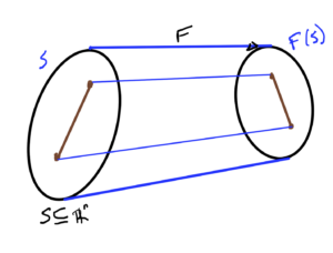
    \end{equation}is convex. Such a mapping is sketched in fig. 14.


fig. 14. Mapping functions of sets.

References

[1] Stephen Boyd and Lieven Vandenberghe. Convex optimization. Cambridge university press, 2004.