New video (on Google’s CensorshipTube):
-
- Click here to watch the video on the Odysee platform.
- [Click here for a PDF version of this post (and supplementary notes for the video.)]
- Look below for a wordpress version of this post (and supplementary notes for the video.)
Exact system.
Recall that we can use the wedge product to solve linear systems. For example, assuming that \( \Ba, \Bb \) are not colinear, the system
\begin{equation}\label{eqn:cramersProjection:20}
x \Ba + y \Bb = \Bc,
\end{equation}
if it has a solution, can be solved for \( x \) and \( y \) by wedging with \( \Bb \), and \( \Ba \) respectively.
For example, wedging with \( \Bb \), from the right, gives
\begin{equation}\label{eqn:cramersProjection:40}
x \lr{ \Ba \wedge \Bb } + y \lr{ \Bb \wedge \Bb } = \Bc \wedge \Bb,
\end{equation}
but since \( \Bb \wedge \Bb = 0 \), we are left with
\begin{equation}\label{eqn:cramersProjection:60}
x \lr{ \Ba \wedge \Bb } = \Bc \wedge \Bb,
\end{equation}
and since \( \Ba, \Bb \) are not colinear, which means that \( \Ba \wedge \Bb \ne 0 \), we have
\begin{equation}\label{eqn:cramersProjection:80}
x = \inv{ \Ba \wedge \Bb } \Bc \wedge \Bb.
\end{equation}
Similarly, we can wedge with \( \Ba \) (from the left), to find
\begin{equation}\label{eqn:cramersProjection:100}
y = \inv{ \Ba \wedge \Bb } \Ba \wedge \Bc.
\end{equation}
This works because, if the system has a solution, all the bivectors \( \Ba \wedge \Bb \), \( \Ba \wedge \Bc \), and \( \Bb \wedge \Bc \), are all scalar multiples of each other, so we can just divide the two bivectors, and the results must be scalars.
Cramer’s rule.
Incidentally, observe that for \(\mathbb{R}^2\), this is the “Cramer’s rule” solution to the system, since
\begin{equation}\label{eqn:cramersProjection:180}
\Bx \wedge \By = \begin{vmatrix} \Bx & \By \end{vmatrix} \Be_1 \Be_2,
\end{equation}
where we are treating \( \Bx \) and \( \By \) here as column vectors of the coordinates. This means that, after dividing out the plane pseudoscalar \( \Be_1 \Be_2 \), we have
\begin{equation}\label{eqn:cramersProjection:200}
\begin{aligned}
x
&=
\frac{
\begin{vmatrix}
\Bc & \Bb \\
\end{vmatrix}
}{
\begin{vmatrix}
\Ba & \Bb
\end{vmatrix}
} \\
y
&=
\frac{
\begin{vmatrix}
\Ba & \Bc \\
\end{vmatrix}
}{
\begin{vmatrix}
\Ba & \Bb
\end{vmatrix}
}.
\end{aligned}
\end{equation}
This follows the usual Cramer’s rule proscription, where we form determinants of the coordinates of the spanning vectors, replace either of the original vectors in the numerator with the target vector (depending on which variable we seek), and then take ratios of the two determinants.
Least squares solution, using geometry.
Now, let’s consider the case, where the system \ref{eqn:cramersProjection:20} cannot be solved exactly. Geometrically, the best we can do is to try to solve the related “least squares” problem
\begin{equation}\label{eqn:cramersProjection:120}
x \Ba + y \Bb = \Bc_\parallel,
\end{equation}
where \( \Bc_\parallel \) is the projection of \( \Bc \) onto the plane spanned by \( \Ba, \Bb \). Regardless of the value of \( \Bc \), we can always find a solution to this problem. For example, solving for \( x \), we have
\begin{equation}\label{eqn:cramersProjection:160}
\begin{aligned}
x
&= \inv{ \Ba \wedge \Bb } \Bc_\parallel \wedge \Bb \\
&= \inv{ \Ba \wedge \Bb } \cdot \lr{ \Bc_\parallel \wedge \Bb } \\
&= \inv{ \Ba \wedge \Bb } \cdot \lr{ \Bc \wedge \Bb } – \inv{ \Ba \wedge \Bb } \cdot \lr{ \Bc_\perp \wedge \Bb }.
\end{aligned}
\end{equation}
Let’s look at the second term, which can be written
\begin{equation}\label{eqn:cramersProjection:140}
\begin{aligned}
– \inv{ \Ba \wedge \Bb } \cdot \lr{ \Bc_\perp \wedge \Bb }
&=
– \frac{ \Ba \wedge \Bb }{ \lr{ \Ba \wedge \Bb}^2 } \cdot \lr{ \Bc_\perp \wedge \Bb } \\
&\propto
\lr{ \Ba \wedge \Bb } \cdot \lr{ \Bc_\perp \wedge \Bb } \\
&=
\lr{ \lr{ \Ba \wedge \Bb } \cdot \Bc_\perp } \cdot \Bb \\
&=
\lr{ \Ba \lr{ \Bb \cdot \Bc_\perp} – \Bb \lr{ \Ba \cdot \Bc_\perp} } \cdot \Bb \\
&=
0.
\end{aligned}
\end{equation}
The zero above follows because \( \Bc_\perp \) is perpendicular to both \( \Ba \) and \( \Bb \) by construction. Geometrically, we are trying to dot two perpendicular bivectors, where \( \Bb \) is a common factor of those two bivectors, as illustrated in fig. 1.
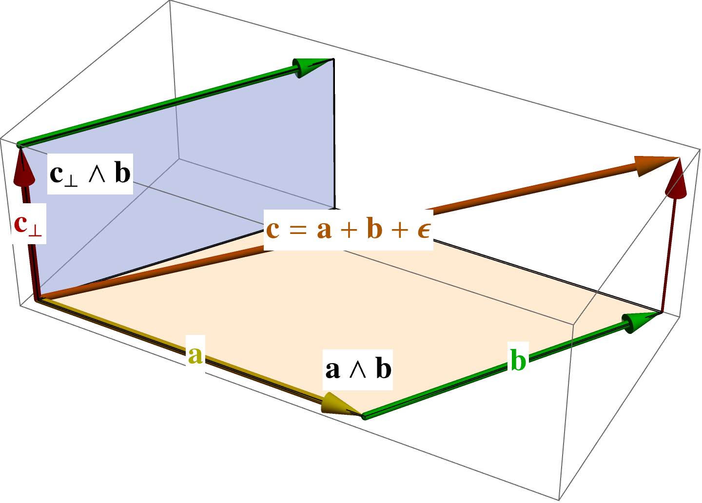
fig. 1. Perpendicular bivectors.
We see that our least squares solution, to this two variable linear system problem, is
\begin{equation}\label{eqn:cramersProjection:220}
x = \inv{ \Ba \wedge \Bb } \cdot \lr{ \Bc \wedge \Bb }.
\end{equation}
\begin{equation}\label{eqn:cramersProjection:240}
y = \inv{ \Ba \wedge \Bb } \cdot \lr{ \Ba \wedge \Bc }.
\end{equation}
The interesting thing here is how we have managed to connect the geometric notion of the optimal solution, the equivalent of a least squares solution (which we can compute with the Moore-Penrose inverse, or with an SVD (Singular Value Decomposition)), with the entirely geometric notion of selecting for the portion of the desired solution that lies within the span of the set of input vectors, provided that the spanning vectors for that hyperplane are linearly independent.
Least squares solution, using calculus.
I’ve called the projection solution, a least-squares solution, without full justification. Here’s that justification. We define the usual error function, the squared distance from the target, from our superposition position in the plane
\begin{equation}\label{eqn:cramersProjection:300}
\epsilon = \lr{ \Bc – x \Ba – y \Bb }^2,
\end{equation}
and then take partials with respect to \( x, y \), equating each to zero
\begin{equation}\label{eqn:cramersProjection:320}
\begin{aligned}
0 &= \PD{x}{\epsilon} = 2 \lr{ \Bc – x \Ba – y \Bb } \cdot (-\Ba) \\
0 &= \PD{y}{\epsilon} = 2 \lr{ \Bc – x \Ba – y \Bb } \cdot (-\Bb).
\end{aligned}
\end{equation}
This is a two equation, two unknown system, which can be expressed in matrix form as
\begin{equation}\label{eqn:cramersProjection:340}
\begin{bmatrix}
\Ba^2 & \Ba \cdot \Bb \\
\Ba \cdot \Bb & \Bb^2
\end{bmatrix}
\begin{bmatrix}
x \\
y
\end{bmatrix}
=
\begin{bmatrix}
\Ba \cdot \Bc \\
\Bb \cdot \Bc \\
\end{bmatrix}.
\end{equation}
This has solution
\begin{equation}\label{eqn:cramersProjection:360}
\begin{bmatrix}
x \\
y
\end{bmatrix}
=
\inv{
\begin{vmatrix}
\Ba^2 & \Ba \cdot \Bb \\
\Ba \cdot \Bb & \Bb^2
\end{vmatrix}
}
\begin{bmatrix}
\Bb^2 & -\Ba \cdot \Bb \\
-\Ba \cdot \Bb & \Ba^2
\end{bmatrix}
\begin{bmatrix}
\Ba \cdot \Bc \\
\Bb \cdot \Bc \\
\end{bmatrix}
=
\frac{
\begin{bmatrix}
\Bb^2 \lr{ \Ba \cdot \Bc } – \lr{ \Ba \cdot \Bb} \lr{ \Bb \cdot \Bc } \\
\Ba^2 \lr{ \Bb \cdot \Bc } – \lr{ \Ba \cdot \Bb} \lr{ \Ba \cdot \Bc } \\
\end{bmatrix}
}{
\Ba^2 \Bb^2 – \lr{ \Ba \cdot \Bb }^2
}.
\end{equation}
All of these differences can be expressed as wedge dot products, using the following expansions in reverse
\begin{equation}\label{eqn:cramersProjection:420}
\begin{aligned}
\lr{ \Ba \wedge \Bb } \cdot \lr{ \Bc \wedge \Bd }
&=
\Ba \cdot \lr{ \Bb \cdot \lr{ \Bc \wedge \Bd } } \\
&=
\Ba \cdot \lr{ \lr{\Bb \cdot \Bc} \Bd – \lr{\Bb \cdot \Bd} \Bc } \\
&=
\lr{ \Ba \cdot \Bd } \lr{\Bb \cdot \Bc} – \lr{ \Ba \cdot \Bc }\lr{\Bb \cdot \Bd}.
\end{aligned}
\end{equation}
We find
\begin{equation}\label{eqn:cramersProjection:380}
\begin{aligned}
x
&= \frac{\Bb^2 \lr{ \Ba \cdot \Bc } – \lr{ \Ba \cdot \Bb} \lr{ \Bb \cdot \Bc }}{-\lr{ \Ba \wedge \Bb }^2 } \\
&= \frac{\lr{ \Ba \wedge \Bb } \cdot \lr{ \Bb \wedge \Bc }}{ -\lr{ \Ba \wedge \Bb }^2 } \\
&= \inv{ \Ba \wedge \Bb } \cdot \lr{ \Bc \wedge \Bb },
\end{aligned}
\end{equation}
and
\begin{equation}\label{eqn:cramersProjection:400}
\begin{aligned}
y
&= \frac{\Ba^2 \lr{ \Bb \cdot \Bc } – \lr{ \Ba \cdot \Bb} \lr{ \Ba \cdot \Bc } }{-\lr{ \Ba \wedge \Bb }^2 } \\
&= \frac{- \lr{ \Ba \wedge \Bb } \cdot \lr{ \Ba \wedge \Bc } }{ -\lr{ \Ba \wedge \Bb }^2 } \\
&= \inv{ \Ba \wedge \Bb } \cdot \lr{ \Ba \wedge \Bc }.
\end{aligned}
\end{equation}
Sure enough, we find what was dubbed our least squares solution, which we now know can be written out as a ratio of (dotted) wedge products.
From \ref{eqn:cramersProjection:340}, it wasn’t obvious that the least squares solution would have a structure that was almost Cramer’s rule like, but having solved this problem using geometry alone, we knew to expect that. It was therefore natural to write the results in terms of wedge products factors, and find the simplest statement of the end result. That end result reduces to Cramer’s rule for the \(\mathbb{R}^2\) special case where the system has an exact solution.